Introduction

I wanted to talk a little about how we are going to do manage and estimate the sensor measurements on board the STM32F4 uC. The goal of this algorithm will not only be to give an accurate measurement of the current state of the flora but it should enable us to understand the health of the flora and the environment within a certain probability. A lot of mathematics are involved in this algorithm. I'm going to be using concepts in differential equations (ODE and PDE) as well as some probability and statics. If you're just interested how we 'built' this thing you might want to move on but if you really want to see the inner workings of what we are doing to make our on-board measurements it's going to be discussed here. So, I'm going to lay it all out and if there are questions you can email me or ask them in the comments and I'll do my best to answer. First I'm going to talk a little about the model and how I derived the model. This will yield the final state space formulation. With the state space described I'll then describe the algorithm we are going to use to estimate our measurements and fuse our sensor information. Lastly, I'll put it into some Matlab simulation and we'll see how it looks when we simulate the algorithm with some real life data. (one note: I know there are not a lot of Matlab fans out there because you have to pay for it but it's what I used in college. Someday I'll port all this over to Octive but for now you're stuck with it...) I'm working on implementing the actual algorithm in the STM32F4 in C but that might take longer than this phase of the project so at least I want to talk about what we are doing and how it is a novel, scientific way to measure the health of flora.

The Model

A model in this case is a mathematical representation of how the system behaves. Many systems will have some inputs and outputs. In our case the system is the environment of the flora we are monitoring. Before the system can be modeled we need to understand a little bit about how it behaves. There are three different, measurements we are taking: light, temperature and humidity. I took some data for an environment where the flora is being kept. This data is shown below:

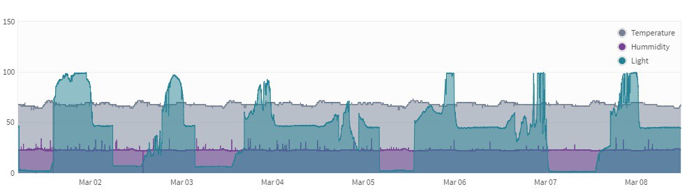
Light is independent of temperature and humidity. Humidity tends to depend on temperature but in a closed environment these can be treated as independent variables. Furthermore all of these variables are slow moving and a little noisy. The sensors we used to take these measurements are:

Light Sensor: Light Sensor Specs: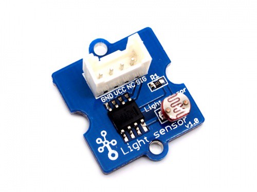

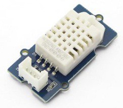
Temperature & Humidity Sensor: The famous DHT11!

These sensors all report discrete values at discrete time intervals. This means we will need to be working with discrete time models. There are a few ways to break down this system. We have the water molecules and air temperature and different aspects of light (i.e. wavelength, reflectivity, transitivity ect...) we could account for in the model. I'm concerned if I take this approach the model will become too difficult to calculate and the data won't be useful.

Instead we can observe that the temperature mostly stay in the same space and are only moved around by a few external forces such as me walking in and out of the room, it raining outside or the cat playing with the sensors. For this reason we can use a discrete "Nearly Constant Position" (NCP) model for the humidity and temperature measurements. The temperature measurement looks like there is some regular movement so if the NCP model doesn't really match the output then we'll switch to the NCV model. I may break down these measurements and look at the frequency content if there is time but for now this is what we'll use. Here's how the NCP model works:

In continuous time the model state is as follows:

Based on the data above we can then say the continuous state equations is:

and the continuous output equation is:

where K is the constant temperature and humidity the room is set to. K can be calculated by taking the average of the first 10 samples.

So now let's change this to a discrete state space model. Before we do this lets clearly define the states A,B,C,D:

Since in the Z domain the C and D matrices do not change all we need to do is calculate the A and B matrices. To do this we evaluate x(t) at discrete times:

and looking at the derivative of the state with the zero order hold of (k+1)T. T=300 because we are going to report every 5 minutes:

Now you can do some calculus and break the integral up into two parts and you'll end up with something like this:

Where

Now the output state pretty much unchanged:

You can calculate the actual values with an inverse Laplace transform...or use Matlab:

[Ad,Bd]=c2d(A,B,T)

Now the actual values for the states are as follows.

The light measurements show a little bit different system. This system is moving at a somewhat regular rate with lots of disturbances. This looks something that can be modeled with a discrete "Nearly Constant Velocity" (NCV) model. Here's how this model works. The setup is the same as above except we are measuring the position and the velocity at which the light changes:

Everything is the same but there are no constants with the light model as the swing is between the max value, 0 and the min value 100. So the discrete state space is as follows:

I omitted the D Matrix in this case because there is nothing forcing the output to a certain value. These are also the preliminary values. When I do the simulations I'll tweek them and pull some more data from our server to see if they are robust for different indoor environments.

Now that we have are state spaces we can have a lot of fun. We can check for things like controllability and observability. So we have two different models: the NCP for temperature and humidity and the NCV for light. We'll need to make two different measurement estimates for these models and have these interact. We can generate different types of estimation systems and that is just what we will do in the next post.