Introduction

In the last post we saw there were two types of models for the system: NCP and NCV. The light measurements were modeled as an NCV type system while the temperature and humidity measurements were modeled as an NCP type system. We have some values for these systems and a brief description on how we came up with the first guess values. In this section we discuss the algorithm we use to estimate the measurements from the sensors. I thought about this a little more and I think the temperature and humidity measurements could also be modeled as an NCV type system and the light measurements, at times could look like an NCP type system. There are a few different tools/filters/algorithms to estimate measurements. I'm going to use a Kalman filter for this this estimation. Furthermore I'm going to use an Interacting Multiple Model Kalman Filter (IMM-KF). The reason that I'm using one of these filters is because:

1. The measurements that we wish to track has two significantly distinct modes of operation.
2. The measurements act like NCV for a period of time, then NCP for another period of time.

The IMM-KF operates multiple Kalman filters in parallel, and systematically mixes state and covariance calcuations each filter to make a composite state estimate and covariance. It is nifty. A much better source than myself for this type of algorithm can be found here:

Mazor, E., Averbuch, A., Bar-Shalom, Y., and Dayan, J., “Interacting multiple model methods
in target tracking: A survey,” IEEE Trans. Aerospace and Electronic Systems, 34(1), Jan. 1998, 103–123.

Before I get into this too much more I want to acknowledge Dr. Greg Plett at UCCS for a lot of these ideas as well and the great notes that he provides to his classes.

So what does this IMM-KF ultimately do? It calculates a probability mass function for the tendency for the system to be operating within a given state. This means that we need to give an probably of transition matrix for each mode. So in mathematical terms specific to the project:

Where mk is the mode at time k. Before we get too deep into the IMM-KF lets go over the Kalman filter.

The Kalman Filter

I've linked the Wikipedia page above to Kalman filters for a deeper understanding but before I move on to how the IMM algorithm makes an estimation I need to at least go over the Kalman filter algorithm at a high level. This filter makes a three key assumptions about the system.

1. We assume that the system dynamics are linear and that it has a PDF that is Gaussian in nature. Most real world systems are not perfectly linear but when I look at the data from our initial measurements I think there are many features of a linear system + noise.
2. The system can be modeled in the state space form:

3. We also assume that the noise processes wk and vk are random mutually uncorrelated white Gaussian with zero mean and covarance matrices in the follow in format:

and

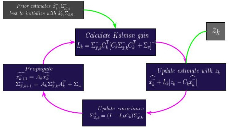
We make these assumptions knowing real systems are never truly linear but it is these algorithms still work really well. It may also comfort you (it comforts me at least) to know that the Kalman filter is the most optimal minimum-mean-squared-error and maximum-likelihood estimator filter you can use for a linear system-but good luck proving this to yourself. So based on these assumptions we can implement the Kalman filter. The Kalman filter calculation can be broken down in to six (easy?) steps. Only an description is given here of what is going on with the key equations. You'll be able to see the mathematics at work in the code, hopefully:

1. State estimate time update

This step calculates the current system state using past measurement information. Typically this means the system will need to be 'initialized' and measured with out any estimation before the Kalman filter is started.

2. Error co-variance time update:

This step calculates a the error covariance estimation of the state prediction. The most recent covariance estimate is calculated then propagated forward in time.

3. Estimate system output

This is the most important step in the Kalman filter estimation process because it generates the real world information that is useful. The result of this step is the best estimate the output given the output equation of the system model, and our best estimate of the current system state.

4. Estimate the Kalman gain matrix

The computation of the gain matrix is the most defining aspect of Kalman filtering and distinguishes the algorithm from other estimation methods. The purpose for calculating covariance matrices is to be able to update the gain matrix. The gain matrix is time-varying. This means it adapts to give the best update to the state estimate based on present conditions.

5. State estimate measurement update

The output estimate is what we expect the measurement to be, based on our state estimate at the moment. So we take the actual measurement and determine what is unexpected or new in the measurement. This is called the innovation. It can be due to an inaccurate system model, state error, or sensor noise. Or maybe all of these. This new information updates the state, but it is weighted according to the value of the information it contains.

6. Error covariance measurement update

The uncertainty of the state estimate has decreased after the measurement update.

Here is a diagram of what this looks like:

There is a lot more to this than what I have here. I cannot possibly document it all in one log. However I'll post the code for the model in the previous log and if there are more questions please put them in the comments and I'll answer them the best I can.

Interactive Multiple Model Kalman Filter

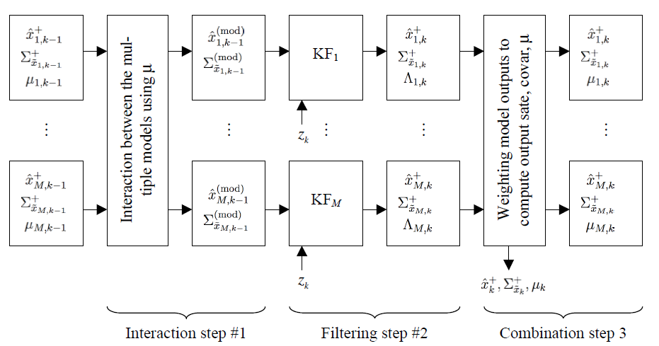
Once the basics of the Kalman filter are understood the IMM-KF is a few small steps from implementing away. A lot of the mathematic rigor is skiped here but you can look at the code in the next log to see how it works or ask me in the comments. The IMM-KF takes three high-level steps per iteration:

Step 1: interaction between the filters

The estimates and covariances from the 2 independent KFs (from the prior time step) are blended together to produce the inputs to the 2 independent KFs for the current time step. First, compute the conditional probability. Then blend together all state outputs from the prior step according to the probability that they could have contributed to the state at this time step.

Step 2: the individual filter update

After the interaction step, one time step for each of the 2 Kalman filters is executed. Both filters output the present state and covariance estimate for that mode, as well as the tendency of the present measurement given that the environment state is in the NCV mode.

Step 3: combination of filter information, yielding the output information.

Lastly, combine the results of the NCP and NCV Kalman filters for an overall environment state estimate and a probability distribution on the mode random variable. First compute the probability of being in NVC mode at time k. Next, calculate the filter output as a mixture of the individual filter estimates, according to the tendency of the environment being in the mode of that filter. Then, the state is computed as a weighted combination of the individual filter state estimates.

Here is a diagram of what this looks like (again credit for this image goes to Dr. Greg Plett from his notes at UCCS):

So, this is the algorithm we're implementing on board the STM32F4 to measure the enviroment of a particular fauna. These states along with the measurements and the measurement estimates are sent to a cloud server for further processing. This enables a high level of resolution in environments where multiple SunLeaf modules are used and very good resolution in environments where only SunLeaf one module is being used. Furthermore, this is typically a very fast algorithm for estimation and can also be implemented in higher bandwidth systems such as autonomous vehicle control systems and fun stuff like that.