 Kuldeep Singh Dhaka
What is FFT?
Wikipedia says (Fast Fourier transform):
A fast Fourier transform (FFT) algorithm computes the discrete Fourier transform (DFT) of a sequence, or its inverse.
Im not going to bombard you with mathematical details (its for another day ;).
What we are today going to do is, capture some real electrical signal with Box0 and visualize it.
There are alot number of education video on Fourier transform on the Internet (example: Youtube).
So, here are some plot that i captured with the code i wrote (code at the end of page).
Sine wave (15.6 KHz)![]()

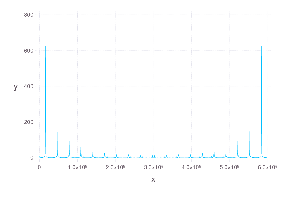
Square wave (15.6 Khz)
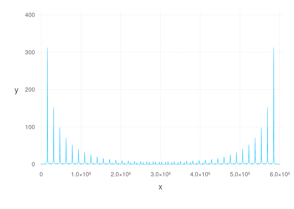
Saw tooth wave (15.6 Khz)
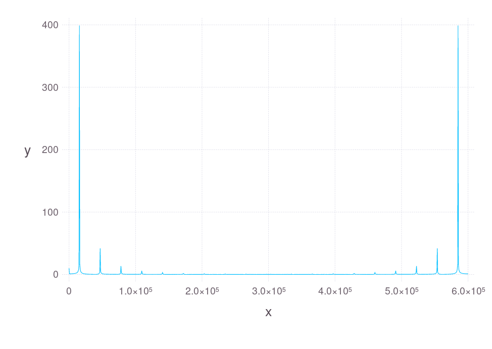
Triangular wave (15.6 KHz)
Python Code
import box0
import numpy as np
import matplotlib.pyplot as plt
import scipy.fftpack

##### PART 1 - Capture

# Allocate resources
dev = box0.usb.open_supported()
ain0 = dev.ain()

# Prepare AIN0 for snapshot mode
ain0.snapshot_prepare()

# Read data from AIN0
bitsize, sampling_freq = ain0.bitsize_speed_get()
data = np.empty(1000, dtype=np.float32)
ain0.snapshot_start(data)

# Free the resources
ain0.close()
dev.close()

##### PART 2 - Process

# perform FFT on captured data
fft_amp = np.abs(scipy.fftpack.fft(data))
fft_freq =  np.linspace(0, sampling_freq, len(fft_amp))

##### PART 3 - Visualize
fig, ax = plt.subplots()

# Show the time domain results (unable to show both plot at once - fix later!...never ;)
#time_x = np.linspace(0, len(data) / sampling_freq, len(data))
#ax.plot(time_x, data)

# Show the frequency domain results
ax.plot(fft_freq, fft_amp)

plt.show()
Julia Code
import Box0
import Gadfly

##### PART 1 - Capture

# Allocate resources
dev = Box0.Usb.open_supported()
ain0 = Box0.ain(dev)

# Prepare AIN0 for snapshot mode
Box0.snapshot_prepare(ain0)

# Read data from AIN0
bitsize, sampling_freq = Box0.bitsize_speed_get(ain0)
data = Array(Float32, 1000)
Box0.snapshot_start(ain0, data)

# Free the resources
Box0.close(ain0)
Box0.close(dev)

##### PART 2 - Process

# perform FFT on captured data
fft_amp = abs(fft(data))
fft_freq =  linspace(0, sampling_freq, length(fft_amp))

##### PART 3 - Visualize

# Show the time domain results (unable to show both plot at once - fix later!...never ;)
#time_x = linspace(0, length(data) / sampling_freq, length(data))
#Gadfly.plot(x=time_x, y=data, Gadfly.Geom.line)

# Show the frequency domain results
Gadfly.plot(x=fft_freq, y=fft_amp, Gadfly.Geom.line)
Note: Though you see – the time domain signal is ideal (mathamatically),
the noise from enviroment and inherit limitation of the signal generator and analog input,
the readed signal is not same as the ideal one.
So it will have minor difference from the “ideal” (mathamatically expected) plot.
Note: The graphs show data above sampling frequency ÷ 2.
You will see: symmetry (called “folding”) around the Nyquist frequency.
Read more on this Wikipedia article
Note: Examples were run in Jupyter Notebook
Note: You can use Box0 – Box0 Studio (Function generator) to generate signal with easy to use GUI.
Hope you like the nerdy post!
Originally posted on https://madresistor.com/blog/fft-and-box0/
Discussions
Become a Hackaday.io Member
Create an account to leave a comment. Already have an account? Log In.