Maxwell Coil

I've decided to use a Maxwell coil to calibrate the sensor(s) on the scanner. Early experiments have shown that the datasheet scale values are rough estimates of the true sensor scales, and calibration will be necessary to obtain acceptable accuracy. The choice of a Maxell design over the simpler Helmholtz coil was motivated by size constraints. For a given physical size coil, the field inside a Maxwell design is uniform over a larger volume - with 3D printed coil forms, this allows larger usable field volumes for a given size printer.

The Maxwell coil design uses three axial windings to produce a nearly uniform magnetic field near the center of the device. This is useful for sensor testing and calibration for two reasons: the field at the center of the coil is easily calculated from first principles (no magnetic calibration required - accurate current measuement is all that's needed), and the uniformity of the field allows for small errors positioning the sensor inside the coil. Unlike the better-known 2-coil Helmholtz design, detailed analysis of the Maxwell design appears to be largely missing from the web, so I did the math and present it here.

The geometry of the 3-coil design is as shown in this figure (NI is the number of ampere-turns of current through the windings):

We are primarily interested in the field at the center of the device - this is the sum of fields generated by the three separate windings. The on-axis field for a single-turn coil of radius R, carrying a current I amperes is derived here:

The easiest way to build a Maxwell coil is to use 64 turns of wire in the center, with 49 on each end, and I assume this construction in the analysis. Using the open-source computer algebra package wxMaxima, derivation of the formula for the total field from the three windings is straightforward:

assume(R[0] > 0);
R[1] : R[0] * sqrt(4/7);
z[1] : R[0] * sqrt(3/7);
B[z] : \mu[0] * I * R^2 / (2 * (R^2 + z^2)^(3/2));
64 * ev(B[z], R = R[0], z = 0) + 2 * 49 * ev(B[z], R = R[1], z = z[1]);

where the magnetic permeability of free space is defined to be:

The permeability of air differs by less than one part per million from this value.

There's an approximation implicit in these calculations: we assume the turns of wire in each winding are all in the same physical location, when in reality each winding has a non-zero length and width. For "small" windings, this is a decent approximation. In a next iteration, I'll expand these calculations to cover more realistic coils with layered windings of non-zero size. In practice, it may not matter.

I created an initial 3D-printable parametric design in OpenSCAD for the coil. Here's an image of the current iteration, printed with a 40mm radius:

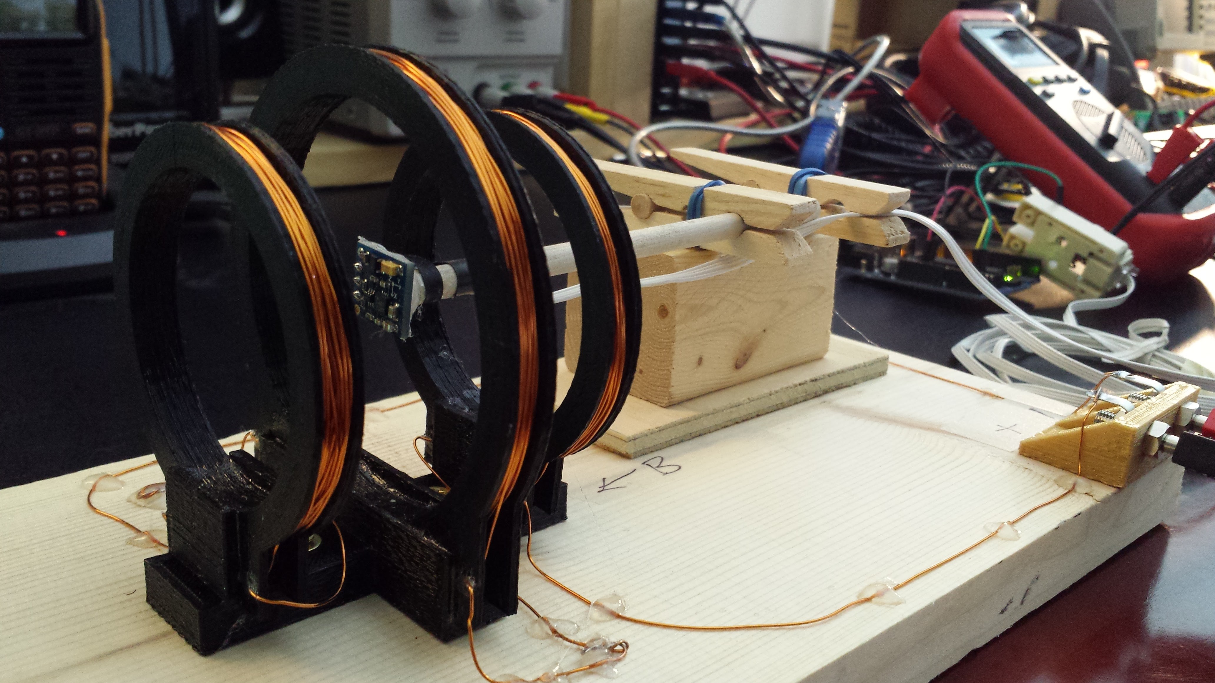
In this build, the coil was scramble-wound with 24-gauge magnet wire. In the next iteration, I'll use proper layered windings, and add extra spars to the form design to keep the coils parallel. All the parts on the board are non-magentic, including brass screws and modified clothes pins hacked with dowels and rubber bands in place of steel springs. The DC resistance of the coil is around 3 ohms, although I didn't bother looking for my Kelvin clips to make an accurate measurement.

Constant-Current Driver

To drive the coil, I prototyped a simple constant-current driver with coarse and fine controls. Here's the circuit:

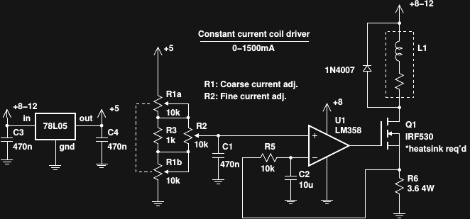
I had a bag of surplus linear stereo potentiometers, so I used the unusual arrangement for coarse and fine controls - the fine knob has 1/10 the range of the coarse. You could alternatively use the other op-amp in the LM358 package to sum voltages from single-gang coarse and fine potentiometers. I also had a bag of 2W 1.8-ohm resistors, so I used two of them in series as a current sense resistor. The large value allows the resistors to dissipate some of the excess power when driving the coil with mid-level current to reduce the thermal load on Q1. A DMM is inserted in series with the coil to measure the current. Driving a power MOSFET this way is fraught with peril; the high inter-electrode capacitances along with the coupled inductance of the coil and haphazard power leads are a recipe for instability. R5 and C2 keep the circuit from oscillating wildly: there's no elegant design here, it's the "big hammer" approach. A more refined version will be needed on the scanner for sensor calibration.

Here's an image of the driver prototype. The fan helps keep things cool, but must be kept away from the coil to avoid disturbing the field.

HMC5883L Results

My early testing of the popular HMC5883L compass sensor indicated that it produces erroneous results in strong fields, reporting small values instead of saturating at full-scale. Armed with a decent field coil, I decided to re-test this sensor to verify the earlier findings. The graph sums it up nicely:

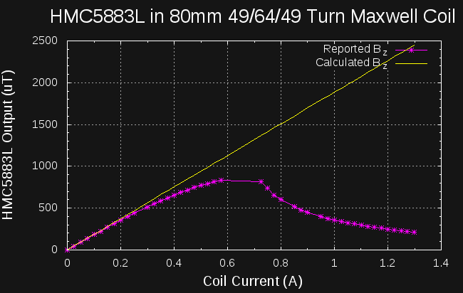
The magenta points are reported by the HMC5883L (corrected for the zero-current field from our fair planet), while the yellow line is the field calculated for the Maxwell coil from the equation derived earlier. I ran similar experiments using both Adafruit's driver library and my own driver, and I'm confident this is not a software bug. In defense of the HMC5883L, the datasheet does list +/- 800 μT maximum range, and the output does saturate for field values of approximately 1100 - 1400 μT, but then starts to report garbage in-range values. The deviation from linearity at the high end of the "usable" range is also cause for concern, but could be calibrated out.

At first, I wondered if my driver circuit or something about the coil could be to blame for these results: maybe the field really does dip like that. Then, I plotted the x- and y-axis field components reported by the sensor on the same graph:

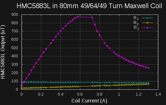
While I did a good job lining up the x-axis of the sensor orthogonal to the coil's field, I was off a little bit in the y-axis, so a small component of the z-axis field is actually picked up by the y-axis sensor. This component shows that the generated field really is linear over the entire current range, and the z-axis values are bunk.

I tried another HMC5883L breakout board. Same thing. This part was my first integrated magnetometer, and we've had several good years together, but it's time to move on.

Next Up

I wanted to get results for the Melexis MLX90393 into this log, but writing the driver is taking a little longer than expected. I'll get there...