 Ted Yapo
Offset Calibration (Duh!)
Sometimes it takes me a while to "get it." Unfortunately, in this format "a while" may be several build logs. This is one of those cases. The original sensor I was using, the HMC5883L, is intended as a compass sensor. Calibration of compass sensors is a well-studied problem, and information about how it works and how to perform it abounds. I had initially dismissed using a compass calibration procedure for the scanner since it only calibrates ratiometric accuracy (the relative scaling of the x-, y-, and z-axes) - exactly what you need for a compass, but not terribly useful for absolute field measurements. In the usual procedure, a large number of measurements are taken with the sensor in random orientations in the geomagnetic field. Plotted in 3-space, the measured field vectors lie on an off-center ellipsoid. Calculating the transformation required to make it a sphere gives you the relative sensitivities of the three axis sensors, while centering the sphere yields the offset. Exactly the offset I need to program the MLX90393 temperature compensation. I think combining a modified "compass calibration" for offsets with some field-coil measurements for scale calibrations will probably work. I'll be exploring this, and will post the results once I have something usable.
Scans!
I got the original demo code re-factored to the point that I can make new scans now. I also wrote field-line integration code in JavaScript so it can run live in a browser, and performance really isn't too bad. For now, I'm using simple Euler integration, but I found this paper on particle tracing in vector fields which explains a higher-order Runge-Kutta method which I will implement going forward. Then there's the topic of interpolation method; for now, I'm just using a simple trilinear interpolation, but I'm going to look into other methods to see if they can provide more accurate results. In any case, here's a low-resolution test scan of a small permanent magnet, captured with only 7x13x13 samples:
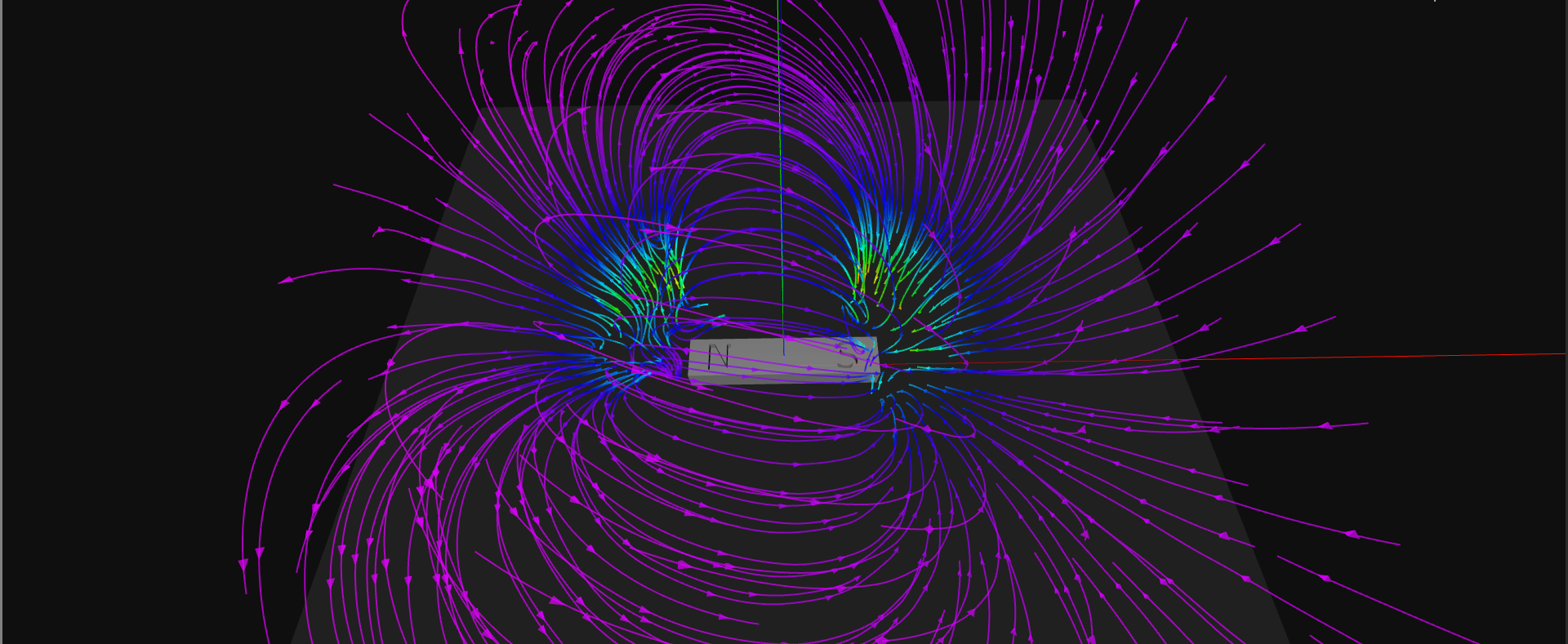
This visualization was done with no calibration whatsoever - no baseline scan, and no offset or scaling from the raw MLX90393 data. It's not numerically accurate, but qualitatively it looks like I'd expect - field lines in loops from north to south. I made a quick model of the magnet in OpenSCAD - this kind of model will be useful when scanning around items: the path-planning code can use such models to avoid collisions with the scanning probe. You can see me sneaking in to measure the magnet during this video of the scan. Remember, don't put your hands inside the printer while it's running. The video is sped up - for now, the scanning is very slow, taking about 20 minutes for this scan, but I think this can be improved quite a bit.
Watching the scan is a little like watching grass grow. I wanted to show it, however, to illustrate the type of magnetic "clutter" one typically finds in a 3D printer: stepper motors and steel rods and frame. How much does that affect the scan? I'm starting to find out. Here's an identical baseline scan taken with the magnet removed:
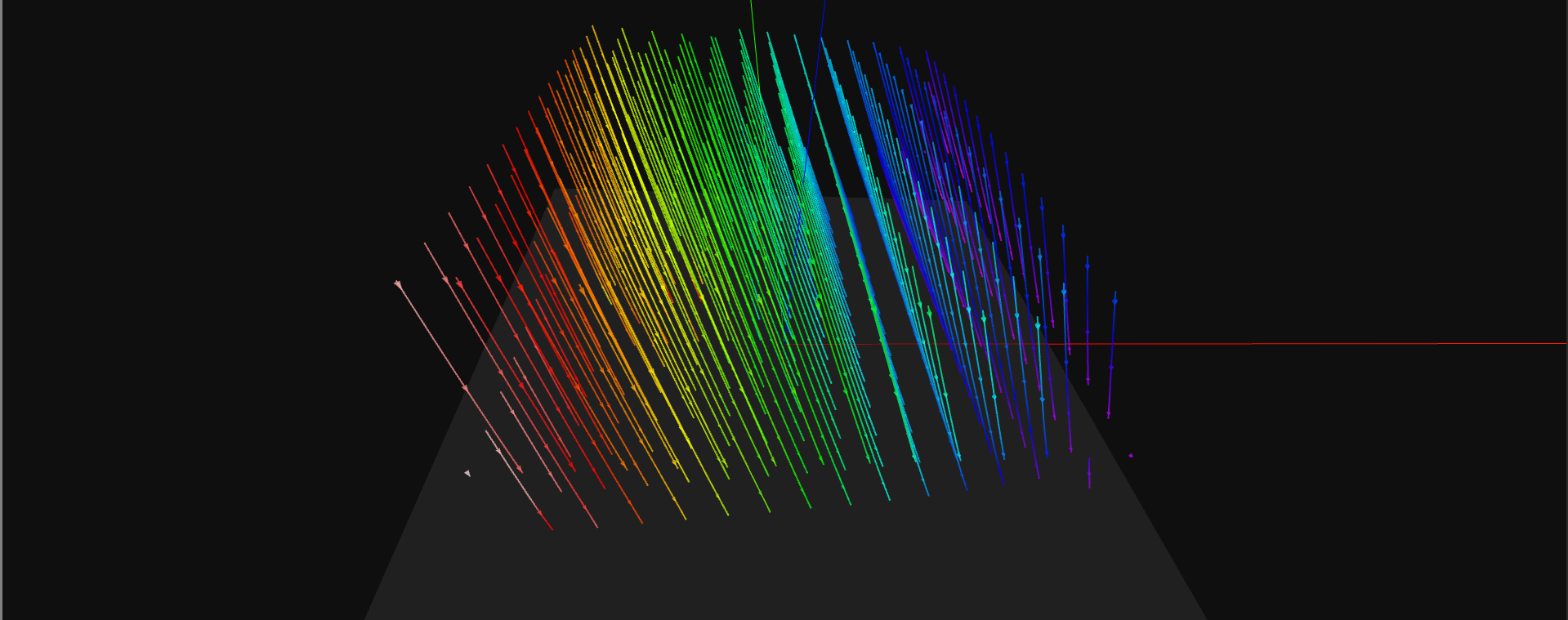
The colors aren't on the same scale between the two plots; the code currently stretches for maximum dynamic range. The baseline, which should consist just of sensor offset and the geomagnetic field, has a range of 141-228 μT, while the bar magnet shows a range of 13-11,485 μT. The interesting thing about the baseline scan is that the field appears to be fairly uniform, except for a slightly stronger field on the negative-x (left) side of the volume. Is that the influence of the stepper motor on the upper left of the video? I'm not sure yet. What appears to be the case is that this baseline is repeatable - I've seen similar fields with each "empty" scan. I haven't diff'ed baseline scans yet to get a quantitative comparison, but so far, it looks like you could correct for this quite easily. The code isn't quite where it needs to be to apply such a correction, but that's the next step.
For very precise scanning, I can imagine taking a baseline scan before and after the real scan to check for repeatability.
Next Up
The big pieces appear to be in place now. I have a variety of things that need work to make this an accurate, reliable, and reproducible system, but clear directions for each. These include converging on a design for the scanning probe, finalizing the calibration procedure, and putting the remaining 20% into a software release (which takes 80% of the time, of course...). Some sort of universal probe mount is also required (and I can't use magnets). After that, path planning, allowing scanning much closer to objects is the next big step. Along the way, I have a growing list of things I want to scan...
Discussions
Become a Hackaday.io Member
Create an account to leave a comment. Already have an account? Log In.
How did you track and pair your coordinates with a MLX90393 measurement? I'm making a similar project using Universal GCode Sender to send GCode commands to my printer and I have my MLX90393 sending back measurements when I ping it. I'm stuck figuring out how to get my current XYZ position and pairing that with a measurement. Thanks!
Are you sure? yes | no
I didn't get a notification for this message, so am just reading it now. I send gcode from python, so there is no buffering. After a move command, I read the sensor. I found that I didn't have to wait long for the printer to move to position before I could read a value.
Are you sure? yes | no