Ted Yapo
-
Yet Another Calibration Log
06/30/2016 at 19:27 • 2 commentsI've been in contact with Melexis regarding calibration and temperature compensation of the MLX90393. They're evidently rationing their application engineers and suggested I contact DigiKey, where I purchased the eval board. DigiKey immediately put me in touch with one of their engineers, who was very eager to help, but set my expectations that he may not have much more luck with Melexis than I had. We shall see. This calibration issue is keeping me up nights, so I'm charging ahead anyway.
Helmholtz Coil
While the Maxwell coil I wound previously is nifty, its better-known cousin, the Helmholtz coil, is much better documented, and using it eliminates one more variable from the experiment.
@jetty has the excellent #Highly Configurable 3D Printed Helmholtz Coil project, which is a very thorough design in OpenSCAD, but is more geared to larger designs with weaker fields, so I decided to create my own. I'll admit to a little "not invented here" syndrome, but the two applications really are different enough to warrant re-inventing the wheel (coil). Just as an example - @jetty's design as built requires about 600mA of current to produce an Earth-strength field over a large volume, while mine requires about 9mA to do the same in a smaller space. Obtaining the 2 mT fields I'm struggling to get by with would require over 60A of current in the larger design. On the other hand, [jetty's] design is perfect for high-accuracy Earth-strength fields.
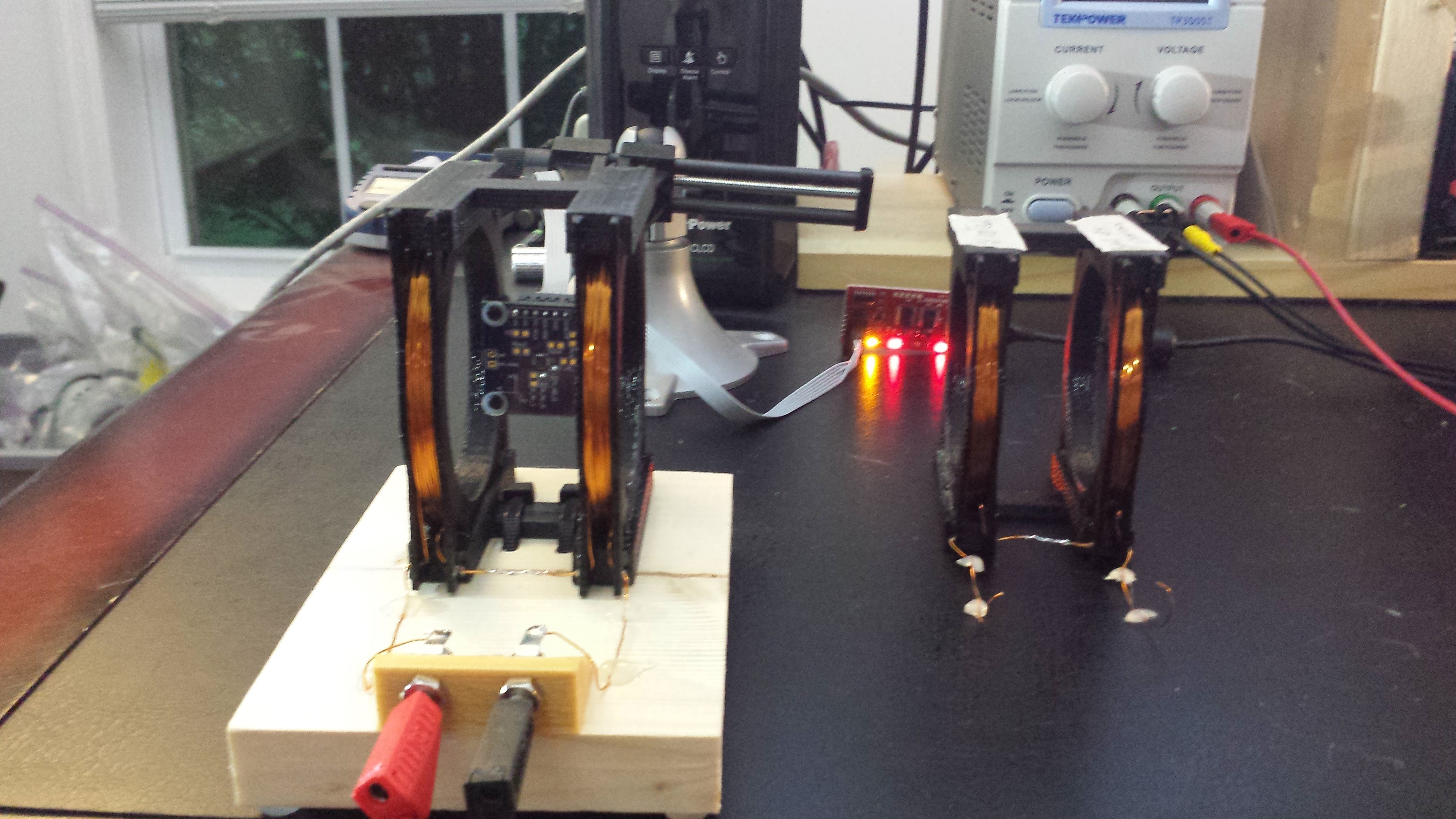
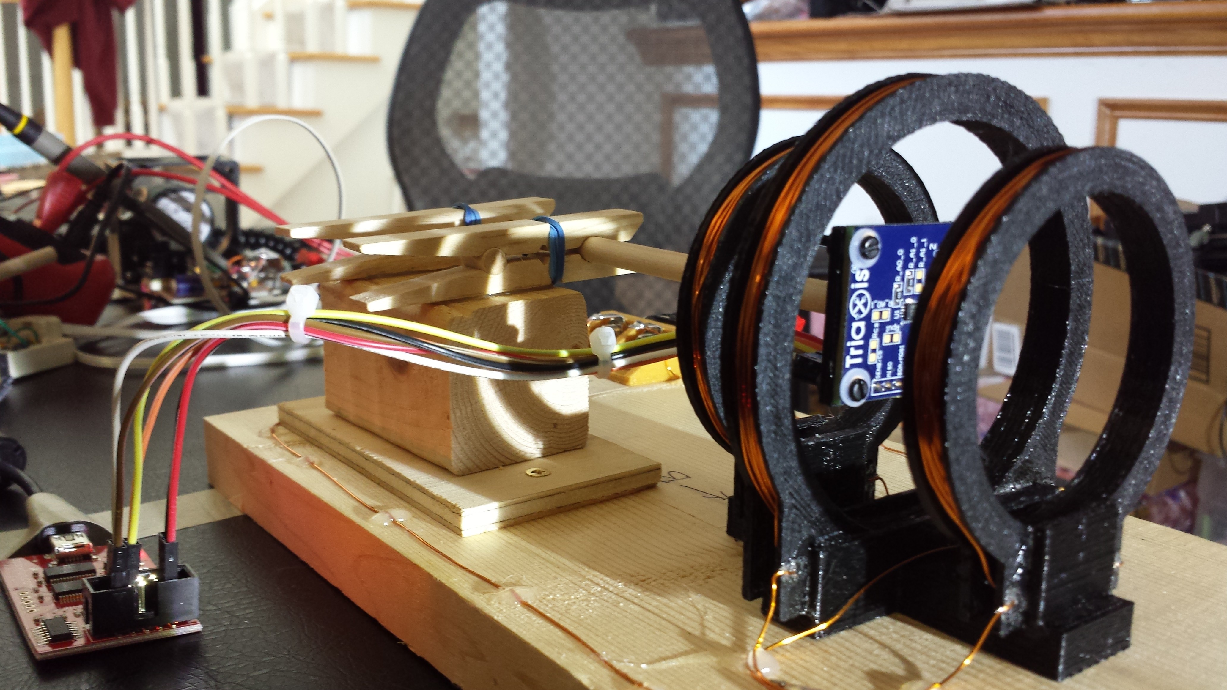
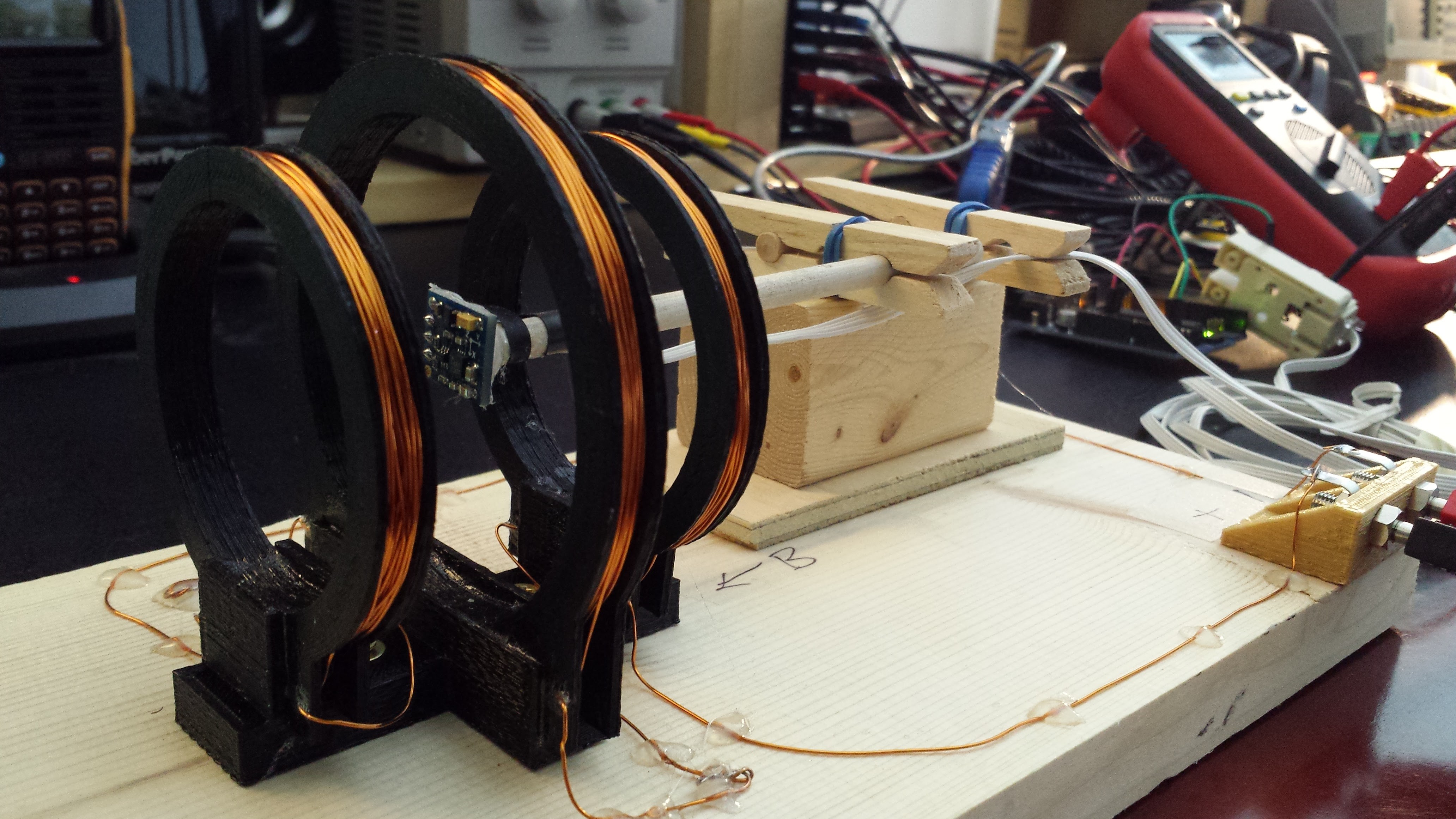
Here's a picture of the two coils I made with my design. They're supposed to have 100 turns of 24 gauge wire on each winding.
![]()
I ended up winding two copies because I got interrupted while wrapping both windings of the first version. I wasn't completely sure if there were exactly 100 turns of wire on either one, so I tested them. My HP3478A meter read 2.173 and 2.223 ohms for the coil resistances, which is troubling. On the other hand, using resistance to evaluate number of turns is problematic - even using 4-wire resistance measurement - since the lead length on the windings is on the order of the length of a turn. I finally measured the inductance of the windings, which is proportional to the square of the number of turns, and relatively insensitive to lead length, so provides a much better measure. Sure enough, the coils read out at 1.524 mH and 1.622 mH, pretty conclusive that the windings are different.
For the second version, I used a python program to count the turns as I very carefully wound them. These windings measured 2.147 and 2.138 ohms and 1.539 and 1.533mH, respectively. I am confident that this coil has exactly 100 turns on each winding.
Analysis
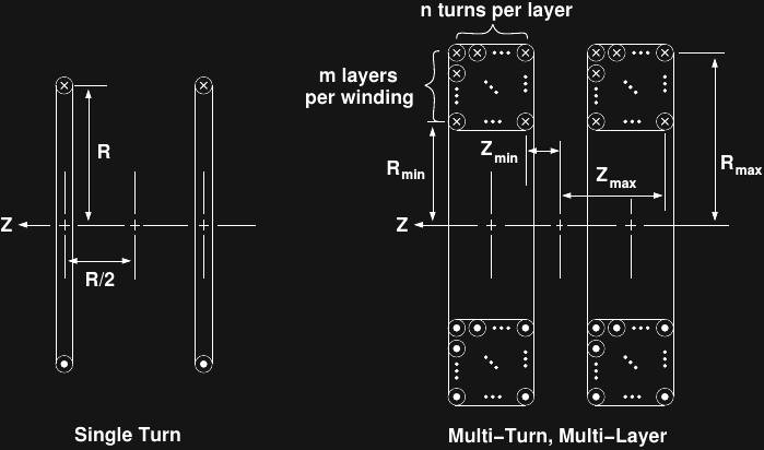
There is a potential problem with this design. The analysis most commonly seen for the Helmholtz coil assumes single conductors in each winding - which is a good approximation for coils like @jetty's, with "small" windings. My design has sizeable windings, however - how much does that complicate matters? I decided to model the "large" windings to find out. I model the "large" windings with m layers of n turns each in a rectangular geometry as shown in the diagram:
![]()
I used wxMaxima again to derive formulas for the field. Starting with the equation for the on-axis field for a single turn:
I first re-derived the formula for the single-turn model:
/* axial field component for a single turn coil of radius R
   carrying current I at distance z */
B_z : \mu[0] * I * R^2 / (2 * (R^2 + z ^2)^(3/2));
/* check that this method produces known formula for single-turn version */
ev(2 * B_z, z = R/2);
Which yields the well-known result:
To evaluate this approximation for the larger-windings, I measured the as-built dimensions and used mean values for the radius and distance:
/* parameters of Helmholtz windings, measured as-built */
z_min : 34e-3/2   /* inner edge of winding */;
z_max : 47e-3/2   /* outer edge of winding */;
R_min : 75e-3/2 /* inner radius of winding */;
R_max : 88e-3/2 /* outer radius of winding */;
n : 10          /* turns per layer */;
m : 10          /* layers per winding */;
/* thin-coil approximation for mean dimensions */
float(2 * 100 * ev(B_z, R = (R_min + R_max)/2,
                        z = (z_min + z_max)/2,
                        \mu[0] = 0.4 * %pi));
Which yields the formula:wxMaxima is just as happy to evaluate the 200-term expression for the multi-turn coil model:
/* sum over layers, turns to get total field */ B_tot : 2 * sum( ev(sum(ev(B_z, R = R_min + (R_max - R_min) * (i-1) / (m-1)), i, 1, m), z = z_min + (z_max - z_min) * (j-1) / (n-1)), j, 1, n);giving:The error in using the single turn formula for this coil is only .05%! Of course, this analysis doesn't address the uniformity of the field within the coil. For a small sensor near the center of the coil, however, I'm satisfied that the coil construction itself isn't introducing a lot of error.
Tangent Magnetometer Test
I read in #Highly Configurable 3D Printed Helmholtz Coil about using the coil and a compass to measure the Earth's magnetic field, then also found this paper describing a similar method, and decided to use the Earth's field to sanity check my coil and calculations.
Using the NOAA's magnetic field estimator, I plugged in my GPS coordinates to obtain (x, y) field values of (19.036 +/- 0.138, 4.604 +/- 0.089) μT, for a total field in the x-y plane of 19.585 +/- 0.164 μT. This is around a 0.8% error bound.
Using the voltage and resistance standards I have available (0.1% and 0.05%, respectively), I measured a calibration for my DMM on the current setting. The uncalibrated error was around 0.3%.
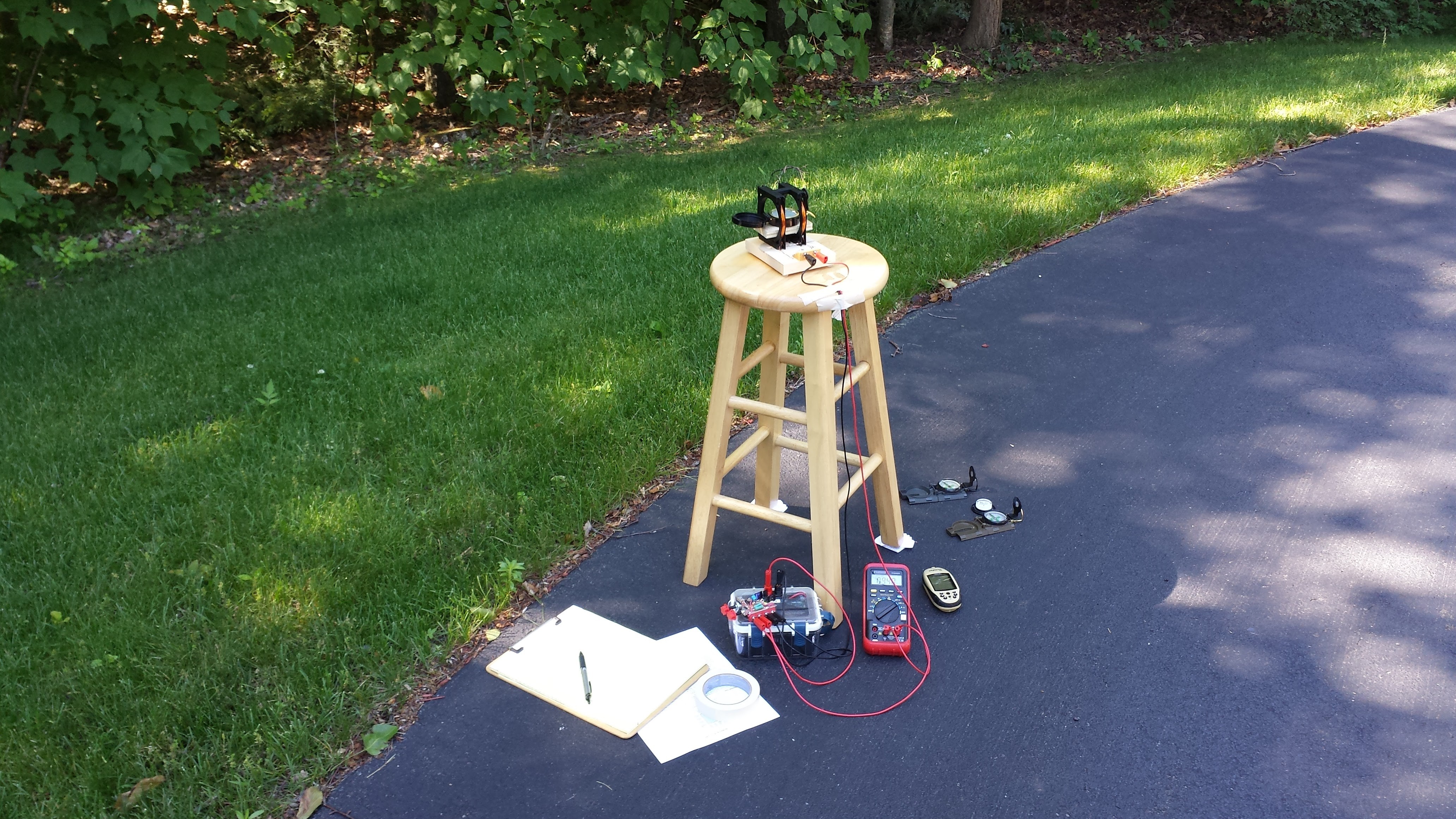
I found a spot in the front yard away from any metal structures to set up the experiment:
![]()
The only compasses I had were really too large relative to the coil, but until some smaller ones arrive, this will have to do. I carefully levelled the platform, since the vertical component of the field at this location is 2.5x that of the horizontal. When the coil is aligned east-west, the ratio of the coil's field to the Earth's is related to the needle's deflection angle by:
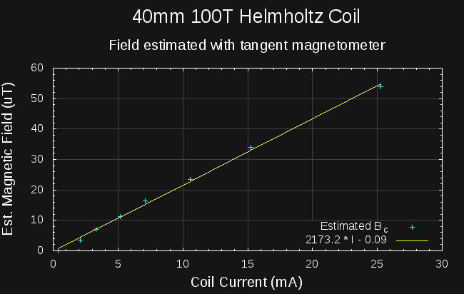
I measured the needle deflection for a series of coil currents, and used the known geomagnetic field to calculate the coil field from this equation. Here's the plot of the estimated field for each current:
![]()
Ignoring the tiny additive constant, the best-fit line reveals an expression for the measured coil field:
This value (2173) is only about 1.8% smaller than the constant calculated from first principles above. I haven't done a thorough uncertainty analysis, but at first glance, it looks like the coil is working as designed, and the field values are probably accurate to a few percent.
MLX90393 Measurements (again!)
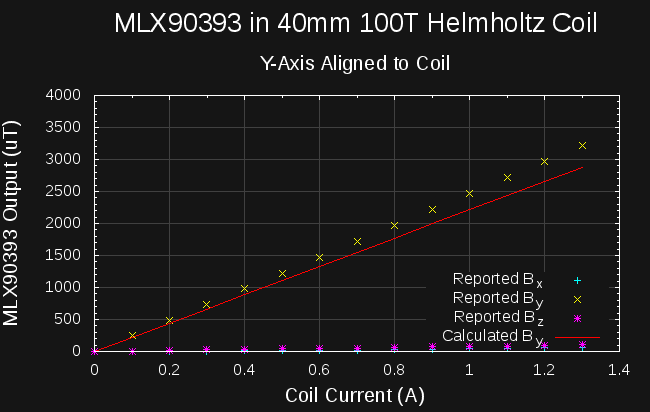
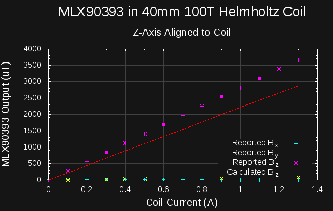
Armed with a validated coil, I measured the 3-component field vectors for the MLX90393 aligned in the coil on each axis:
![]()
![]()
![]()
Using the calculated factor (2213.6) for the Helmholtz coil, and fitting regression lines to the MLX90393 outputs vs calculated field values gives the following scale constants:
x-axis y-axis z-axis 1/1.098 1/1.117 1/1.273 so, the field values reported by the MLX90393 are off by around 10-11% in x and y, and almost 30% in z
You can see, especially in the y-axis plot, that I didn't manage to get the axes precisely aligned; there's some spill of the field into the supposedly orthogonal axes (the MLX90393 lists additional 1% typical cross-sensitivites). Correcting for this isn't trivial, since we don't know the scale factors a priori: if we did, we could just calculate the total field and regress to that. Instead, I just roughly estimated the error using the uncorrected raw values, obtaining bounds of around 0.2% for x, 3.4% for y, and 2.2% for z.
I'll work through the math to come up with a better method for dealing with this error.
The conclusion seems to be that the MLX90393 sensor will need calibration in the scanner. I'm thinking of a small 3-axis coil that can serve double-duty: calibrating the field range of the 3-axes, and aligning the magnetic field vectors in the printer's coordinate system. I haven't discussed the latter issue much, but I've given it a lot of thought, and this seems like the easiest way to get the magnetic coordinate system properly registered with the spatial one.
Next Up
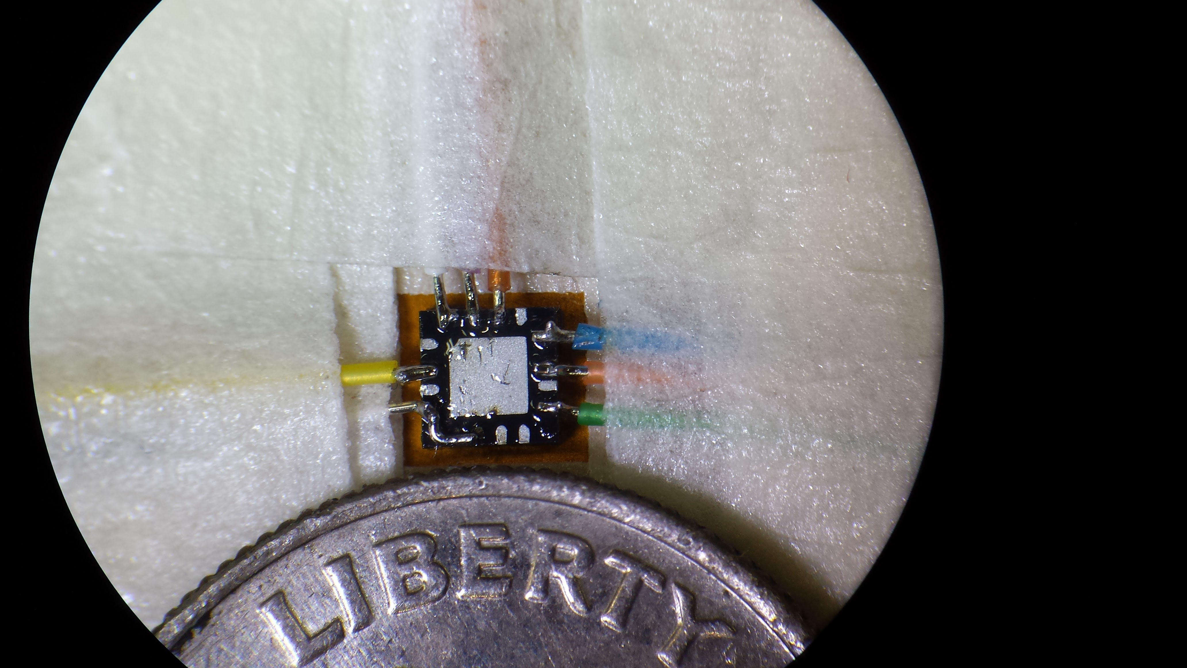
Sleep. It's 02:30 local time. Tomorrow, I'll try out this assembly. I couldn't wait for boards, so I soldered wire-wrap leads to the 3x3mm QFN package directly:
![]()
-
Protecting Your Printer
06/29/2016 at 12:22 • 2 commentsFirst a quick note: I've re-thought my earlier log about ENIG finish. Instead of spreading fear, uncertainty, and doubt about this noble metal finish, I've decided to take a more scientific approach. I'll have my boards fabbed in HASL and ENIG, and see if I can detect any differences in performance.
You Broke My Printer
I really don't want to hear this - ideally because it didn't happen :-) I really don't want to break my printer(s), either. I've developed three lines of defense against damaging expensive printers by using them as scanning magnetometers: kill switches, sacrificial scanning heads, and a safety-conscious scanning protocol enforced in software.
Robot Kill Switches
I'm a firm believer in hardware kill switches. Right at the power source. No matter what coders would have you believe, no software-based kill switch is reliable enough to adequately protect life and property. This is especially true with machines built around current 3D printer controllers, whose firmware buffers up commands to accelerate printing. Sending a "stop" command just doesn't cut it when your printer is breaking itself. I've tried.
Here's a picture of the switches I use for 3D printers and other devices in the shop:
![]()
The first two are simple off-the shelf devices - a power strip and a wired remote switch. The latter is convenient because it lets you keep the switch easily reachable, but the only one I could find is 2-wire, meaning you have to lift the ground connection to use it, which is not ideal. Unable to find a suitable wired switch commercially, I built the third model from an extension cord (cut in half), a heavy-duty outdoor enclosure, and a paddle switch. The large paddle is convenient because you can hit it with your hand or foot or whatever isn't being pulled into the machine at the moment.
If you end up using the scanner being designed here, I highly recommend using a hardware kill switch of some sort. Just in case.
Head Mount Design
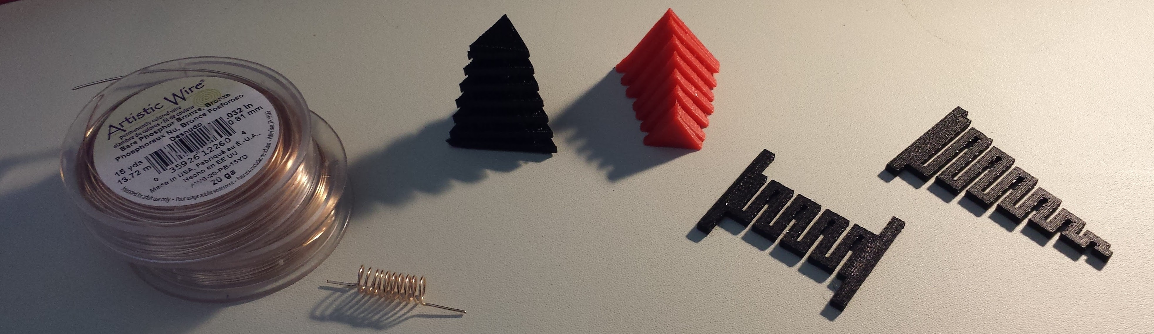
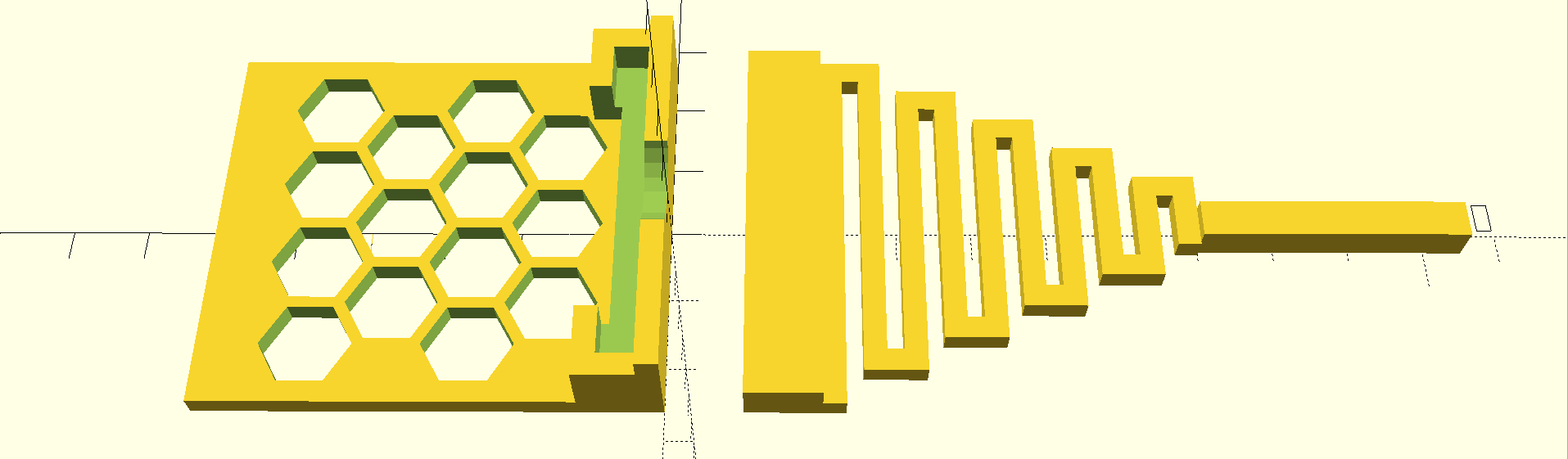
The idea for this project is to avoid any permanent modifications to your printer. While I'm also looking into making a dedicated scanning platform based on printer designs, for now, the focus is on adapting existing printers. In order to protect the printer during scanning, I envisioned a scanning head design combining a spring and shear-pin that would yield if struck gently, but break long before the printer if struck hard. Here are some steps along the evolution of the scanning head design:
![]()
Wanting to avoid ferrous metals in the head design, I started with springs wound of phosphor-bronze wire - the idea was to connect two lengths of wooden dowel with the springs. I soon remembered that using a 3D printer as a scanning magnetometer pre-supposes that the user has a 3D printer (duh!), so a printed design would be ideal. My first experiments with the triangular "3D" springs shown were both interesting and frustrating. Making the springs triangular in cross-section makes them easily printed without support material, but unfortunately, the "weak direction" of the print always ends up along two of the sides, making them too fragile to be useful in this design. I'll post the OpenSCAD file for them anyway, in case somebody can find a way to improve the idea. I finally settled on a flat spring design like the last two - this design keeps the spring in the "strong" printing direction, has a low profile, and prints quickly (good for a sacrificial part). The spring constant and breaking point are both easily changed (but not directly calibrated) by manipulating the shape. My daughter called the tapered version a "tornado spring" - this is the design I ended up using.
My ultimate goal is to come up with a universal mount for attaching the scanning head to any 3D printer. For now, I've settled on simply mounting it on my first test printer - a Solidoodle 3. Here's the design I'm currently testing:
![]()
The Solidoodle head has a laser-cut piece of plywood that makes a convenient attachment point; this mount is press-fit onto that board, then held in place with a piece of adhesive tape. The hexagonal grid is just lightening holes to reduce material used and printing time. The two pieces are designed to be glued together in this first iteration. Since the spring sensor mount also functions as a shear pin and is designed to break, a quick-release mount of some sort will eventually be required. A quick-release probe mount also figures largely in the scanning protocol discussed below.
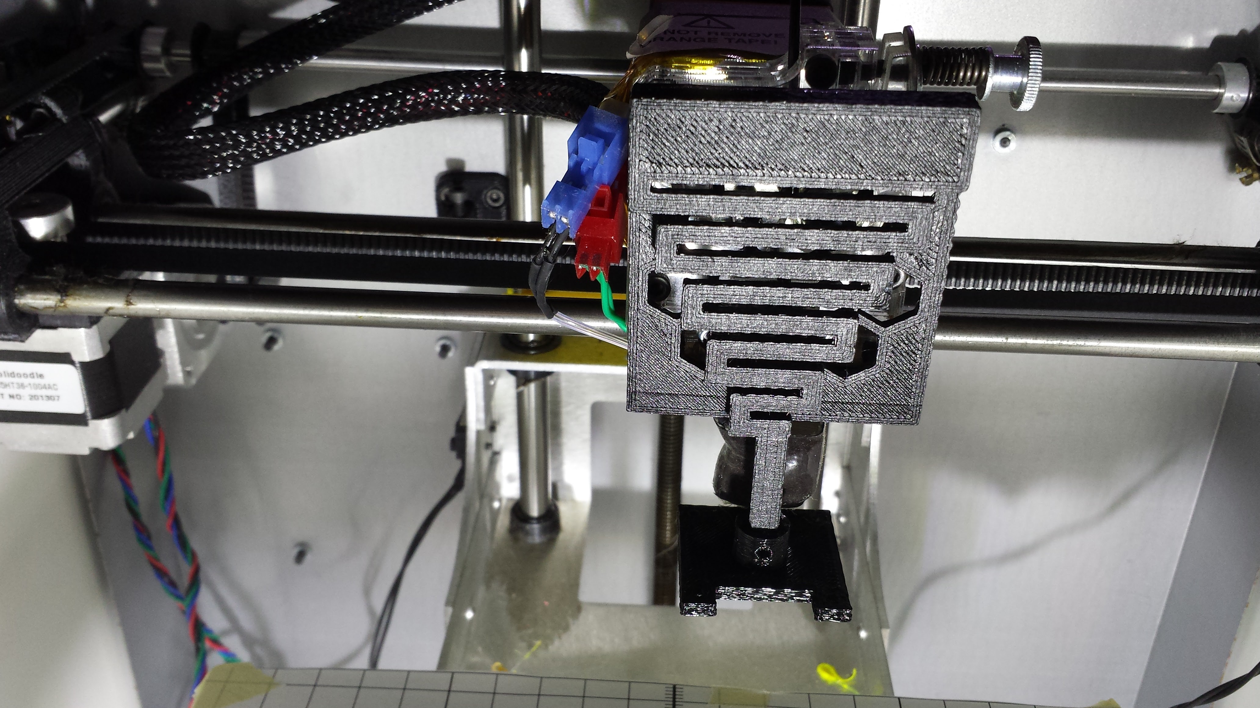
Here's the design mounted on the printer head, along with the mount for the (huge!) MLX90393 evaluation board:
![]()
This head is designed for "Phase 1" of the design, where all scanning takes place above any target object - so clearance to the printer's hotend is not an issue. In latter phases, when scanning inside the bounding volume of targets, the probe will be extended below the nozzle with a longer spring assembly. Even in this version, the scanning head should be a bit lower to provide some extra clearance for the nozzle.
Scanning Protocol
Additive manufacturing robots have an easy time of path planning: they inhabit an empty universe. As soon as a layer is printed, the tool head moves up relative to the work-piece, thus never having to concern itself with avoiding contact with the piece. Subtractive manufacturing robots don't have it so good: there's often a big piece of metal in the center of their world that they must avoid while moving. This is the same problem that will be faced in Phase 2 and beyond of the scanner: path planning algorithms will be required to keep to the scanning head (and printer head itself) from striking the target.
I'm still thinking about the path planning problem, but I've come up with a preliminary scanning protocol to avoid the most obvious causes of object collisions in the scanner, while avoiding modification of the limit switches and other mechanisms of the printer. Here's the step-by-step, starting from the beginning of a scan:
- User enters scan parameters, including bounding volume or 3D model of scanning target
- User is prompted to remove the quick-release detachable probe from the printer, and any scanning target currently on bed
- User acknowledges completion of this task
- Printer homes head (as usual), then moves head to center (x, y) of scan volume, at z-level safely above scanning volume
- User is prompted to mount quick-release probe and arrange scanning target on bed
- User acknowledges completion of this task
- Printer scans over volume, using path planning algorithms to avoid striking target with probe
- When scan is done, printer moves head to original centered position above the target and prompts user to remove target
- User acknowledges completion of this task
- If a baseline scan is desired for calibration, printer performs this baseline scan, then returns to center position
- User is prompted to remove quick-release probe
- User acknowledges completion of this task
- Scan is complete
It sounds like a lot of steps, but they're all common-sense and fairly trivial. Some obviously could be eliminated if a dedicated scanning device were used instead of leveraging an existing printer.
In all the "user acknowledgement" steps, I'm considering using a trivial CAPTCHA-type response like:
Enter "576" to continue:
where the "576" is randomly generated. The idea is to prevent accidental acknowledgements from distracted operators (or cats walking on your keyboard). You'll be able to turn this off.Next Up
I'm continuing tests on the MLX90393 - I've wound a Helmholtz coil (actually two!), worked out some math, and checked the calibration of my current meter to get to the bottom of the scaling issues. I'll report progress soon. I'm also working on two board designs for the probe head, and of course, getting a Phase 1 software release ready.
-
The Problem with ENIG
06/21/2016 at 15:45 • 2 commentsEDIT: I've re-thought this log, and decided to take a more scientific approach to evaluating ENIG finish in this application. See later logs for details.
So, I'm thinking about the sensor design - I need a small PCB to carry the MLX90393, then another remote board to hold a microcontroller (spoiler alert, I'm thinking PIC here), programmable current source for electromagnet experiments, and USB-UART bridge. I naturally started wondering about the nickel used in the ENIG finish on many boards, and what magnetic properties it might impart. Electroless nickel immersion gold (ENIG) plating uses a thin layer of nickel over the copper traces, and a very thin layer of gold over the nickel. Nickel, like iron, is ferromagnetic (but less so): it's attracted to magnets, and can be made into permanent magnets.
To see if an ENIG finish interacted with magnetic fields, I suspended a PCB with ENIG finish from a thread, and tried to attract it with a strong NdFeB magnet, as shown in this video:
The effect is very weak - you can't pick up the board with a magnet or anything like that - but very real. My concern for the sensor head is that the nickel on the board may become magnetized during the scan, skewing the results, or act as a magnetic flux concentrator, distorting the measured field.
I noticed that the MLX90393 evaluation board uses a gold finish of some type, as does the HMC5883L breakout board from Adafruit, although I'm not sure if either finish is ENIG. Have they done the calculations and/or tests to show that this doesn't affect the measurements? Who knows. I don't think I'm going to take any chances, though - it's HASL for the sensor board.
-
MLX90393 Saturation Test
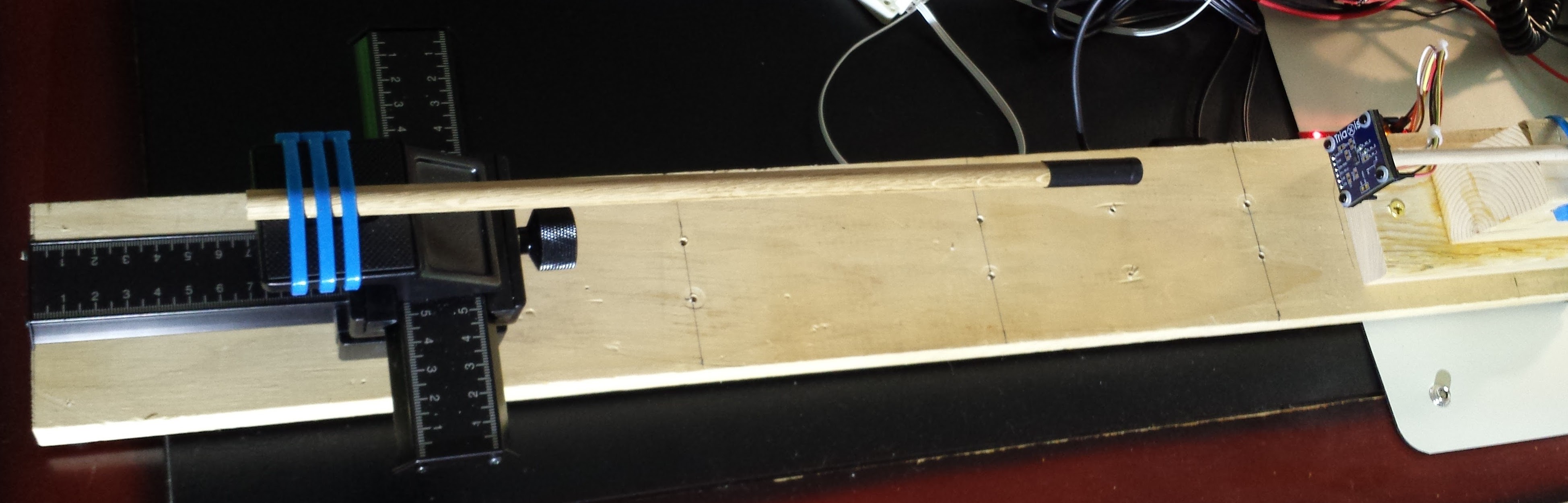
06/21/2016 at 02:43 • 4 commentsI built a simple rig to test for magnetic saturation in the MLX90393 sensor. I happened to have a manual X-Y stage for macro photography, so I used it to move an 8mm NdFeB magnet (of strong but unknown field) near the sensor. Here's a picture of the apparatus:
![]()
The magnet was attached to the end of a 320mm wooden dowel with a length of heat-shrink tubing. The polyolefin tubing I used lists a shrink temperature of 125C, leaving a safe margin to the over 300C Curie temperature of NdFeB, so there's little chance of harming the magnet this way. The magnet/dowel assembly is then lashed to the X-Y stage to allow fine positioning of the magnet relative to the sensor.
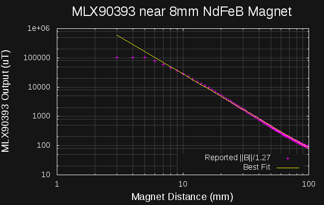
I collected data from 3 to 98mm distance, recording a point every 1mm. The MLX90393 has GAIN_SEL=0 and RES=3, for a maximum full-scale range of 129184 μT according to the datasheet. After applying my empirically determined scale-factor of 1/1.27, this comes out to a little over 100 mT full-scale. The datasheet also states that the sensor starts to enter saturation (i.e. deviation from linearity) at around 50 mT. Here's the data I collected:
![]()
The data points are magenta; the yellow is a best-fit line to extrapolate the true field for small distances. Magnetic fields around a dipole drop off with an inverse power law, the exponent being 2 in the near field, and 3 in the far field. The regressed line here has a slope of -2.53, which seems plausible. The interesting thing about this line is that it shows an extrapolated field strength of approximately 0.6 T at 3mm. Sintered NdFeB magnets have a field strength of between 1.0-1.4T, so this seems reasonable. The MLX90393 output saturates at around 100mT (the full-scale value), and as noted in the datasheet, starts to deviate significantly from linearity at around 50mT.
I'm quite impressed with this sensor! These results would indicate that you could scan to within 6mm or so of the strongest magnets available, and still collect usable data. Closer than that, and the output would saturate, but this is easily detected and flagged in a visualization. I've selected a sensor: time to start designing a tiny board to carry it.
Next Up
I still haven't determined where the 1/1.27 scale factor comes from - I'm going to continue thinking about that. The Melexis web site is back up, and I downloaded their app note about temperature compensation; I should be able to add that to the driver soon. I'm also going to mount this sensor in a 3D printer and get back to what this project is supposed to be about - scanning some fields.
-
First MLX90393 Tests
06/17/2016 at 19:03 • 0 commentsI read about this project on Hackaday this weekend. It's funny - I've read hundreds of Hackaday write-ups, and never really thought about the hours that went into each project until I saw my own up there. Impressive community of hackers. Thanks of course to @Benchoff and the staff there for the visibility and kind words!
Avast, Ye Hackers!
I stayed up late last night and wrote a python driver for the MLX90393 using the SPI binary scripting mode of the Bus Pirate board (from Sparkfun, and of course, [Ian]). One of the difficulties is that the MLX90393 requires a hardware line to signal the master when conversions are done; there's no way for software to poll. This probably makes sense during sensitive magnetic field measurements, since polling by the master could only serve to distort the field. For now, I'm using generous delays set according the the expected conversion times listed in the datasheet. Using the Bus Pirate will probably be good enough until I get the final sensor head designed and built. At least I'm getting data. You can check out the code over at GitHub.
I printed a simple mount to attach the MLX90393 evaluation board to a 1/4" wooden dowel, and found some non-magnetic header pins to solder on the board. The mount holds the EVB with nylon screws and nuts. Here it is in the coil, connected to the Bus Pirate with short jumpers - I'll need to make some longer ones to scan some test fields with this part. As you can see, the EVB is huge (30x30mm), even though the MLX90393 itself is only 3x3mm, and doesn't require any external parts. I'm going to throw in a bypass cap on the final sensor head, even though the datasheet would have you believe it's optional.
![]()
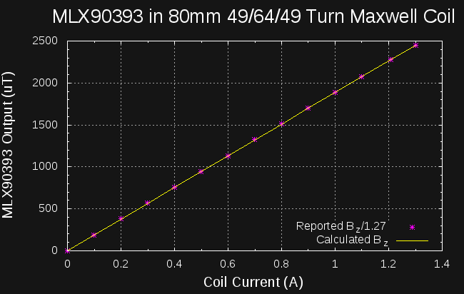
The first data I collected was a repeat of the HMC5883L tests run earlier. Here's the first graph, comparing the reported z-axis component of the field with the field calculated from the current and Maxwell coil dimensions:
![]()
This is more like what we want to see! The scaling is based on calibration values provided in the datasheet: the only correction applied to the data was to subtract off the zero-current reported field (25.87 μt) from all data points. The linearity is clearly there, but the scaling is definitely off. At this point I don't know if:
- the scale factors in the datasheet are incorrect
- my Maxwell coil or calculations are off
- this part just needs to be calibrated before use
To get a better feeling for the issue, I did a regression fit to find the scale factor, and then replotted the data (this assumes the coil is correct):
![]()
Much better. The best-fit scale factor is 1.27, which, maybe out of pure coincidence, is almost exactly one "GAIN_SEL" step in the MLX90393. I've poured over the code and poked around registers for a while now, and can't find where I'm screwing this up. I did find an error in Table 4 of the datasheet (on the same page as the scale factor table), so it's possible the scale factors in the datasheet are also incorrect. Specifically, the offset for the {RES = 3, TCMP_EN = 0} case is 2^14, not 2^15 as shown in the datasheet. I noticed the error after testing with these settings produced clearly wrong values, and I was able to confirm the error in Table 4 by comparing it to the "MLX90393 Getting Started" application note. I haven't found a similar error for the GAIN_SEL parameter, though. Unfortunately, Melexis' web site appears to be in a state of flux: the links to their datasheets and appnotes were broken for the past few days, and today their entire site is 503. When they come back on-line, I'll see what other clues I can dig up.
The driver doesn't implement temperature compensation yet, since I couldn't download the relevant application note, and that information is missing from the datasheet.
In any case, it looks like we have a winner with this sensor - it's nicely linear to the limit of my first calibration set-up.
50mT in a Maxwell Coil?
If I had been paying attention to my own logs, I would have seen this earlier. The maximum full-scale range of the MLX90393 sensor is around 50mT. The field in the Maxwell coil is:
Plugging in 50mT for the field and 40mm for the radius, we find that we need a current of about 26 amps. In the 3-ohm coil, this would dissipate over 2000W, melting the PLA coil form a few seconds before melting the windings themselves. It actually sounds fun, and I do have a pair of 40V Li-ion packs for my electric string trimmer that might be able to produce that much current, but it's not a practical way to test the sensor range...maybe once I have a better coil this one can be sacrificed in the name of science.
What I really want to see is what happens when the MLX90393 is exposed to fields greater than its full-scale range. Does the output saturate at full-scale, or does it fold over and produce bad data like the HMC5883L? I think I'd be OK with calibrating the sensor in the low-end of the range and extrapolating to full-scale calibration as long as the part saturated properly.
To test for full-scale saturation, I'm working on a little rig to accurately position a rare-earth magnet near the sensor. A little more time in the shop and I should be ready to collect some data.
Auto Ranging
The MLX90393 allows for a total of 32 different scale factors. The trade-off being full-scale range vs. precision. Of course, many of the ranges overlap significantly, so you can probably cover the full range with good resolution using just a handful of settings. Unfortunately, the part doesn't do auto-ranging, so that would need to be added to the driver. With the wide range of fields likely to be encountered during "interesting" scans, I think it's probably a requirement.
Next Up
Testing the MLX90393 with a strong magnet, and further sleuthing about the 1.27 scale factor.
-
Sensor Testing
06/16/2016 at 14:55 • 0 commentsMaxwell Coil
I've decided to use a Maxwell coil to calibrate the sensor(s) on the scanner. Early experiments have shown that the datasheet scale values are rough estimates of the true sensor scales, and calibration will be necessary to obtain acceptable accuracy. The choice of a Maxell design over the simpler Helmholtz coil was motivated by size constraints. For a given physical size coil, the field inside a Maxwell design is uniform over a larger volume - with 3D printed coil forms, this allows larger usable field volumes for a given size printer.
The Maxwell coil design uses three axial windings to produce a nearly uniform magnetic field near the center of the device. This is useful for sensor testing and calibration for two reasons: the field at the center of the coil is easily calculated from first principles (no magnetic calibration required - accurate current measuement is all that's needed), and the uniformity of the field allows for small errors positioning the sensor inside the coil. Unlike the better-known 2-coil Helmholtz design, detailed analysis of the Maxwell design appears to be largely missing from the web, so I did the math and present it here.
The geometry of the 3-coil design is as shown in this figure (NI is the number of ampere-turns of current through the windings):
![]()
We are primarily interested in the field at the center of the device - this is the sum of fields generated by the three separate windings. The on-axis field for a single-turn coil of radius R, carrying a current I amperes is derived here:
The easiest way to build a Maxwell coil is to use 64 turns of wire in the center, with 49 on each end, and I assume this construction in the analysis. Using the open-source computer algebra package wxMaxima, derivation of the formula for the total field from the three windings is straightforward:
assume(R[0] > 0);
R[1] : R[0] * sqrt(4/7);
z[1] : R[0] * sqrt(3/7);
B[z] : \mu[0] * I * R^2 / (2 * (R^2 + z^2)^(3/2));
64 * ev(B[z], R = R[0], z = 0) + 2 * 49 * ev(B[z], R = R[1], z = z[1]);
The result (which wxMaxima will even format infor you) is given by:
where the magnetic permeability of free space is defined to be:
The permeability of air differs by less than one part per million from this value.
There's an approximation implicit in these calculations: we assume the turns of wire in each winding are all in the same physical location, when in reality each winding has a non-zero length and width. For "small" windings, this is a decent approximation. In a next iteration, I'll expand these calculations to cover more realistic coils with layered windings of non-zero size. In practice, it may not matter.
I created an initial 3D-printable parametric design in OpenSCAD for the coil. Here's an image of the current iteration, printed with a 40mm radius:
![]()
In this build, the coil was scramble-wound with 24-gauge magnet wire. In the next iteration, I'll use proper layered windings, and add extra spars to the form design to keep the coils parallel. All the parts on the board are non-magentic, including brass screws and modified clothes pins hacked with dowels and rubber bands in place of steel springs. The DC resistance of the coil is around 3 ohms, although I didn't bother looking for my Kelvin clips to make an accurate measurement.
Constant-Current Driver
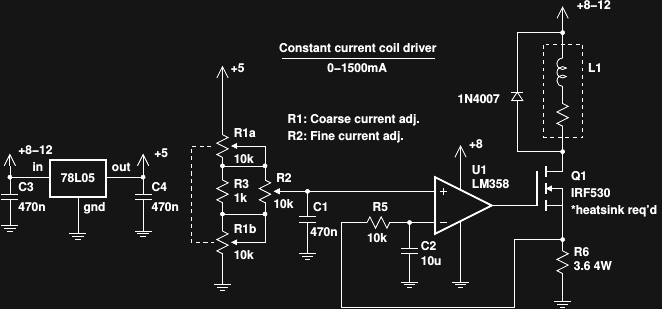
To drive the coil, I prototyped a simple constant-current driver with coarse and fine controls. Here's the circuit:
![]()
I had a bag of surplus linear stereo potentiometers, so I used the unusual arrangement for coarse and fine controls - the fine knob has 1/10 the range of the coarse. You could alternatively use the other op-amp in the LM358 package to sum voltages from single-gang coarse and fine potentiometers. I also had a bag of 2W 1.8-ohm resistors, so I used two of them in series as a current sense resistor. The large value allows the resistors to dissipate some of the excess power when driving the coil with mid-level current to reduce the thermal load on Q1. A DMM is inserted in series with the coil to measure the current. Driving a power MOSFET this way is fraught with peril; the high inter-electrode capacitances along with the coupled inductance of the coil and haphazard power leads are a recipe for instability. R5 and C2 keep the circuit from oscillating wildly: there's no elegant design here, it's the "big hammer" approach. A more refined version will be needed on the scanner for sensor calibration.
Here's an image of the driver prototype. The fan helps keep things cool, but must be kept away from the coil to avoid disturbing the field.
![]()
HMC5883L Results
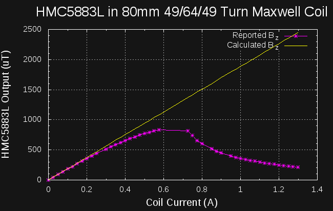
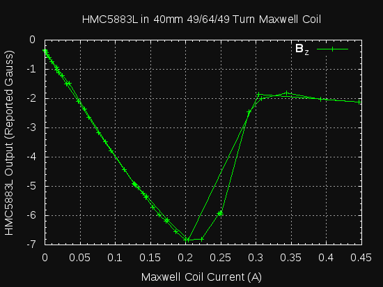
My early testing of the popular HMC5883L compass sensor indicated that it produces erroneous results in strong fields, reporting small values instead of saturating at full-scale. Armed with a decent field coil, I decided to re-test this sensor to verify the earlier findings. The graph sums it up nicely:
![]()
The magenta points are reported by the HMC5883L (corrected for the zero-current field from our fair planet), while the yellow line is the field calculated for the Maxwell coil from the equation derived earlier. I ran similar experiments using both Adafruit's driver library and my own driver, and I'm confident this is not a software bug. In defense of the HMC5883L, the datasheet does list +/- 800 μT maximum range, and the output does saturate for field values of approximately 1100 - 1400 μT, but then starts to report garbage in-range values. The deviation from linearity at the high end of the "usable" range is also cause for concern, but could be calibrated out.
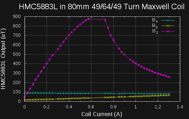
At first, I wondered if my driver circuit or something about the coil could be to blame for these results: maybe the field really does dip like that. Then, I plotted the x- and y-axis field components reported by the sensor on the same graph:
![]()
While I did a good job lining up the x-axis of the sensor orthogonal to the coil's field, I was off a little bit in the y-axis, so a small component of the z-axis field is actually picked up by the y-axis sensor. This component shows that the generated field really is linear over the entire current range, and the z-axis values are bunk.
I tried another HMC5883L breakout board. Same thing. This part was my first integrated magnetometer, and we've had several good years together, but it's time to move on.
Next Up
I wanted to get results for the Melexis MLX90393 into this log, but writing the driver is taking a little longer than expected. I'll get there...
-
Magnetometer Sensor Survey
06/04/2016 at 17:32 • 7 commentsI've thought more about the sensor issue, and it probably doesn't make sense to put this off until a later phase of the project. I'm now fairly convinced I'll need a custom sensor head early, so it makes sense to get a board designed and off to fab. I can code while I wait for the board and parts. But first, let's consider the fields we'd like to measure.
Magnetic Field Strengths
My ideal goal is to be able to measure a range of magnetic field strengths you might find around items we usually associate with magnetism. A comprehensive scale of field strengths can be found on wikipedia. We consider the Earth to have a relatively "weak" field (at 30-60 μT) , and I think fields of this magnitude are a good low bound. As it turns out, there's an active market for sensors to measure fields in this range for use as compasses, yielding noise-limited resolutions of under 1 μT. Probably the strongest fields in common experience are produced by neodymium-iron-boron rare-earth magnets, on the order of 1.4T maximum. This is 45,000 times more powerful than the Earth's field, and easily overwhelms "compass" sensors, which may have full-scale readings on the order of 1000 μT. It adds up to a very wide range. Let's have a look at what we can do with readily available sensors.
Integrated Sensor Roundup
Here's a quick table I put together for the three-axis sensors I could order today from DigiKey or Mouser. I'm not particularly interested in using unobtainium sensors in this project, so I won't consider any you can't buy or make from parts offered by these distributors.
Part # Manufacturer Noise (resolution) (μT) Max. FS (μT) Cost (Qty. 1) LIS3MDL ST Microelectronics 0.32 1600 $1.70 AK8963 AsahiKASEI (0.15) 4900 $3.08 MAG3110 Freescale/NXP 0.25 1000 $1.46 HMC5883L Honeywell 0.2 800 unknown MLX90393 Melexis 0.5 50000 $2.14 Notes:
- Click the part numbers for datasheets
- In cases where RMS noise was listed in the datasheet, I've reported that as a limiting factor, otherwise I've listed the maximum resolution (in parenthesis). All of these are probably noise-limited, so be wary of the parenthesized values.
- For the MLX90393, the noise depends on a settable averaging time parameter. I chose approximately 50ms as a conversion/averaging time for this table.
- I couldn't find an orderable HMC5883L in ten minutes of looking. From the table, I'm not sure the part is best for this project, anyway, despite its popularity in hacker-friendly breakout boards.
The MLX90393 is the clear winner here, at least based on a quick scan through the datasheets. It's positioned as a general-purpose sensor, as opposed to the others, which are fairly compass-specific. Some of the applications they list are rotary and 3D joystick encoders (with permanent magnets), which is pretty interesting in itself. Melexis offers a $20 breakout board at DigiKey, so I'll order one of those to evaluate as a start. It's a shame that a 3x3mm part needs a breakout board so large - I'll definitely need a much smaller custom sensor board/head for the final scanner.
Beyond 50 mT
While the 50 mT maximum range of the MLX90393 is a big step up from the 0.8 mT range of the hacker-favorite HMC5883L, it still falls short of being able to measure fields from powerful permanent magnets. Wikipedia lists 5 mT for typical refrigerator magnets, so they're in, but Nd2Fe14B magnets at 1T or more are still way out of reach. I have three (EDIT: four!) ideas so far for extending the range. In each case, I'm considering adding a secondary sensor for strong fields (of course, the more sensitive sensor will need to survive the strong-field exposure).
Single-Axis Sensors
Single-axis Hall-effect sensors are available for position sensing in stronger fields. From a cursory look, drift with time and temperature might be a problem, since they're not typically aimed at precision measurement applications. I'm going to look further into this.
Magnetic Shielding
By enclosing one of the above sensors in a "soft" iron shield, it should be possible to extend the full-scale range significantly, and it may be possible to accurately calibrate out field distortions caused by the shielding. The idea is that most of the magnetic flux will be contained in the high-μ shield, leaving a smaller field inside for the sensor. I'll have to rig up a quick test with some cast-iron pipe fittings as a shield (too big and probably too magnetically "hard" for use in an actual sensor). One issue with this approach is that the shield will experience forces due to the field while scanning. 3D printers, as opposed to milling machines and the like, are not designed to resist serious forces on the head. This will require some thought.
DIY Sensor
I can't help myself. I prototyped a simple 2-axis fluxgate on a high-μ ferrite core years ago, and was able to crudely sense compass headings. Maybe I can revisit this with a low-μ core for sensing more powerful fields.
"Compensation Coil"
This was the original thought I had - then I forgot it writing up this log - by surrounding the sensor with a 3-axis field coil, a controllable portion of the external field can be "cancelled out" inside the coil. This is known as "active shielding". It suffers from the same problem as the passive shielding described above, namely forces exerted by the external field. Additionally, generating a field strong enough to partially cancel that from a rare-eath magnet won't be easy - and then there are thermal issues to consider (the coils will get hot). The upside to this method is that a single sensor could conceivably be used for both strong and weak fields just by varying the coil current.
Printer Thoughts
I've been looking at 3D printers in a different light recently. It seems that parallel robots (e.g. delta-bots, scara designs) are probably better than serial (e.g. cartesian) 'bots for this type of scanning, since all the stepper motors can be outside the build (scanning) volume. I notice that #low-field MRI settled on a polar-coordinate arrangement to deal with this issue. I'm thinking that out of the typical printing arrangements, a delta-bot designed for a Bowden extruder might be best. I may have to find a cheap delta-bot kit to hack for testing, because unfortunately, serial bots in my lab outnumber parallel designs 3.5 to 0 (the 0.5 is from my unfinished homebrew franken-printer)
-
Proof of Concept
06/02/2016 at 17:35 • 0 commentsResults
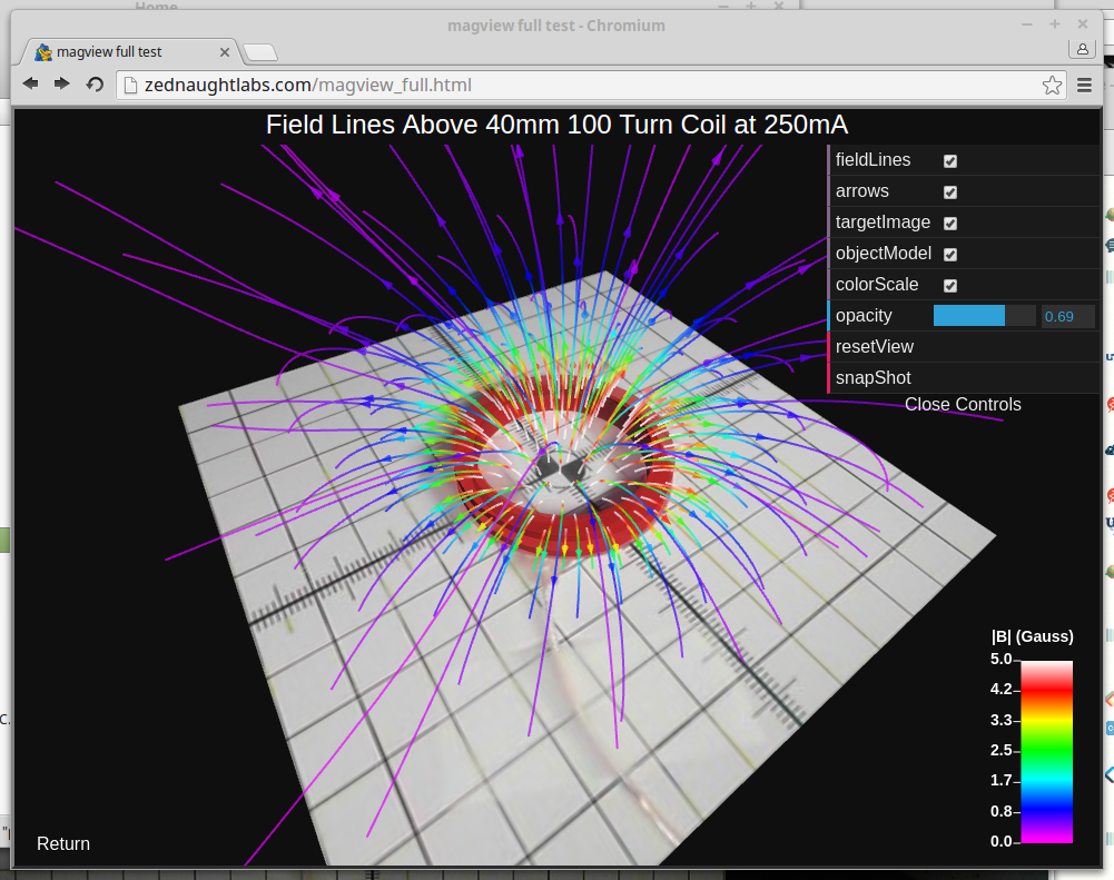
I linked the prototype viewer in the description; but here it is again for completeness:
For anyone who can't run the visualization for some reason, here's a screenshot:
![]()
Software
The first proof of concept used three quick software prototypes:
- Scanner: a python program for controlling the printer and sensor
- Processor: C++ code to apply the calibration, interpolate the data, and generate the field line visualization
- Viewer: WebGL code (and necessary HTML) to display the visualization in a browser
Going forward, I intend to eliminate the second step, and generate the visualizations "on-the-fly" in JavaScript, allowing for a much more interactive exploration of the field.
Hardware
I used my Solidoodle 3 printer as a testbed for this first run. An Arduino Uno responds to serial-port commands from the python "scanner" code and communicates with an Adafruit HMC5883L breakout board over I2C.
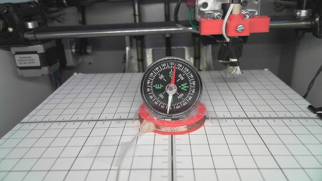
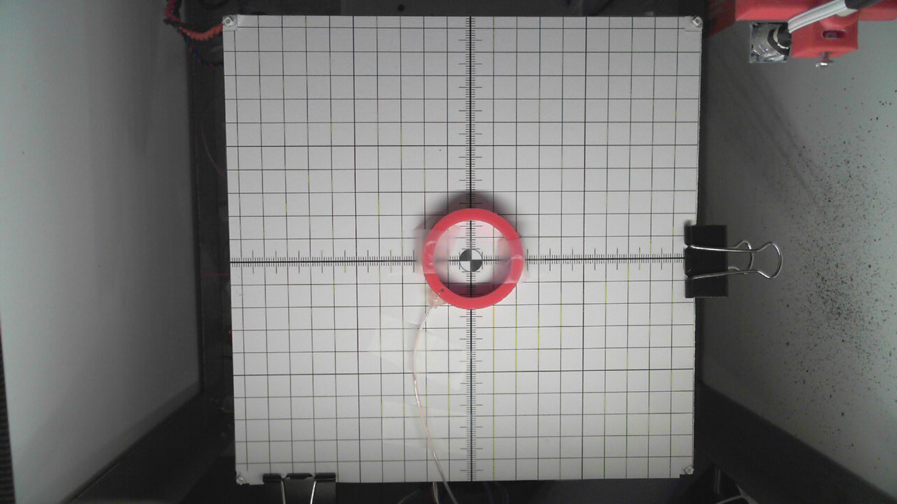
As a first scanning target, I printed a 40mm diameter coil form and wound 100 turns of magnet wire scavenged from an old oscillating fan on it - the wire is approximately 28 gauge. I drove the coil with a constant current of 250mA since this produced a good range of field strength without saturating the sensor. Using a coreless electromagnet for testing makes compensating for external fields easy - take a sample with the coil on, another with the coil off, and subtract. Here's a picture of the setup (I used the compass for a quick check of the field). The scanning head (in the background) is attached to the printer's extruder with a printed clip (in red).
![]()
A printed target sheet was attached to the printer bed, and an overhead image was used to texture-map the 3D model in the viewer. An initial experiment used controlled LEDs (just visible unilluminated at the grid corners) for automatic registration of the 2D image with the 3D model.
![]()
When using a known 3D model for scan boundaries, this type of (2D) printed grid will be used to align the object in the scanner's coordinate system. A PDF file containing the grid with an outline of the object's footprint can be generated - then you simply have to place the object on its 2D footprint.
Anomalies
I noticed some strange behavior with the HMC5883 sensor. The datasheet states:
In the event the ADC reading overflows or underflows for the given channel, or if there is a math overflow during the bias measurement, this data register will contain the value -4096
while this may be true specifically regarding the ADC and math overflows, I found that exceeding the range of the sensor actually generates bad data. At first I suspected the Adafruit code I used to drive the HMC5883 (sorry for the thought, Adafruit, your code is blameless here), but found the same results when I wrote my own driver. Here's what I found in a quick test with the HMC5883 inside a Maxwell coil (which produces a nearly uniform field):
![]()
The results up to about 200mA look pretty good, then things fall apart - the output doesn't saturate as the datasheet initially led me to believe. I ran the current up, then back down looking for a tell-tale hysteresis loop that would indicate something on the board becoming magnetized (the nickel in an ENIG finish? ferrous contacts on SMD passives?), but don't see one in the lower range. The troubling part is the fold-over in the curve. If you measure -2 Gauss, is it really -2, or more like -12? I need to re-run these experiments more carefully and then determine how to proceed. If this data is correct, options include surrounding the sensor with a servo'd "compensation coil" or finding a new sensor, possibly a homebrew fluxgate on toroid cores. For now, I'll be careful not to exceed the maximum range during scans.
3D Magnetic Field Scanner
Capture interactive models of magnetic fields with your 3D printer