In the last log, I briefly mentioned what I think were the problems in my old setup to research the influence of flow speed on the electrical behaviour of electrolytic solutions. In this log, I want to go over these problems and discuss the high-level design choices I made to alleviate them.

The longevity of the measurements

While the measurement itself took 2 minutes, the water was pumped between containers, so it had to be pumped back. I also wanted to flush the setup after each experiment, to make sure measurements couldn’t influence each other. All in all, this could make measurements last up to 10 minutes. This may not seem like much, but please consider that I did three different measurements at each flow speed^[1], and tested at about 10 different flow speeds.

You can see that collecting all the measurements can take quite a long time. And during this time, temperature can vary, salt can precipitate out of solution, and so on. Because of this, there may be deviations introduced in data, which are undesirable.

Also, the longer the measurements, the less you can perform in a given amount of time. Because of this, I only had one data point for every condition. This means that you can’t average out any inherent deviation in your system, which makes for these unclear correlations. Or in scientific terms: the lower the amount of data points, the lower your significance will be.

We can solve this problem by examining the electrical behaviour of the solution at alternating voltages at various frequencies. This technique is called Electrochemical Impedance Spectroscopy, or EIS. It is much faster, while providing some additional information. I will go into more detail in a separate log.

The function fitting did not work to well

In my previous research, I used what is called a least-squares function fit to fit my experimental data to the theoretical behaviour of the solution.

To understand why this is problematic, we must first examine function fitting in closer detail. A function fitting algorithm is an algorithm that you feed a set of points, your data, and a function that has certain parameters, would be a basic example. You then give the function fit a guess for what the parameters need to be. It then tries to find the parameters that will make the function go through the data as well as possible.

The least-squares function fitting algorithm is perhaps the most basic widely-used function fit. It basically just tries to minimise the average distance of the data to the function. However, it has the problem that it tends to find local maximums. This picture illustrates this quite well:

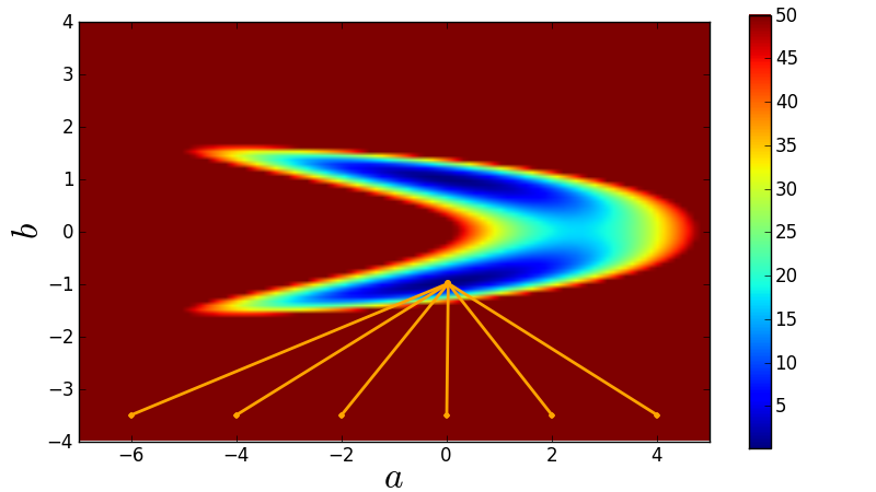
Figure 1: The tendency of a least-squares function fit to find local maximums. From the Python course for MPIA. Copyright 2011, Smithsonian Astrophysical Observatory. Used under a Creative Commons Attribution 3.0 License.

Also, my function had 5 parameters. The more parameters you have, the more difficult it becomes to get a good fit. Needless to say, I had quite a few measurements where the function fit determined that the resistance was very high, while the capacitance was really low, where other measurements where swapped. This made analysis difficult.

I will try to solve this problem by directly calculating the parameters from the data. If I have more data points then needed, I might average the parameters calculated from various samplings of data points together. Whatever I’ll decide, I will probably document it in a log about the software.

The flow speed was not tightly controlled

In my previous research I used a pump to pump the solution through a measurement tube. The pump had no control loop associated with it. Even though it was a pretty strong pump, and hence not influenced by small changes in pressure all that much, it still was a little bit. Because of this, the flow speed wasn’t perfectly constant. Also, due to the mechanics of the pump, it moved the solution with small burst, which also isn’t an ideal constant flow rate. You can see these effects in the graph beneath:

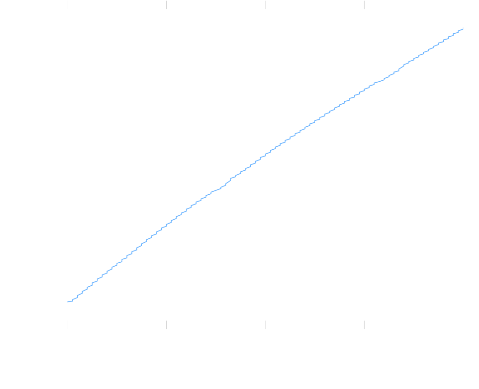
Figure 1: Weight displaced by the pump over time.

Also, the pump may have sucked up some undissolved salt from the bottom of the solution storage container, so that the conductivity of the electrolytic solution varied, which isn’t ideal.

These effects contribute to the noise in the data, which I want to eliminate. So for this incarnation of my test setup, I am not using a pump to pump the solution along the electrodes, but I am moving the electrodes through the solution. Using a linear slider from Actobotics and a stepper motor, the electrode array can be dragged through a basin with the solution. Since the measurements will be much faster, it is possible to use a rather small basin, in fact I’m using a cake tin. This has the added advantage that the whole solution is easily accessible, so that it can be stirred periodically to make sure there is no undissolved salt.

This works because physics has to be the same, regardless of the reference frame. The only thing that matters for us is relative speed, so whether the solution moves along the electrode, or the electrode moves through the solution, as long as the speed at which they move relative to each other is equal, the situations are physically the same.

These were the high-level improvements I’m making that are driving the design. Let’s dive in the electrical details of that design in the next log.

Endnotes

[1] One with the pump of for calibration, one with the stepped pump, and one actual measurement in case you were wondering.