 andrew.powell
So, instead of simply going over the software and hardware, I think it would be more interesting to explain the theory of operation, and then dive into the project’s implementation! I might change this format in future projects. But, for now I think it’s a really awesome format since I find it’s really awesome and/or advantageous to know how something we might see or use everyday often has a strong theoretical background. I hope others find this format as exciting as I do, and I appreciate any kind of feedback if there’s any!
By the way, I want to apologize if the equations are difficult to read due to the background color. I'm still figuring out how to best present certain information!
The Idea: Real-Time Visual Equalizer
All a visual equalizer fundamentally does is display the frequency content of a signal at each instance of time, where frequency content of a signal is simply the same signal whose magnitude changes with respect to frequency. Not sure if there’s an official definition of a visual ( or sometimes graphic ) equalizer, but I think my definition concisely describes what a visual equalizer effectively does.
The Theory: Fun with the Fast Fourier Transform!
But, how does one obtain a frequency spectrum of a signal at an instance of time? Well, one way would be to implement a series of bandpass filters whose center frequencies correspond to the frequencies that I want the visual equalizer to display. If I was going to do an analog implementation of this project, I’m certain my best option would be this approach. Luckily, since I know my target development board consists of both an FPGA and a multi-core processor ( MCP ), my amount of available design options are much greater!
I still could have implemented a bunch of bandpass filters, however I wanted to ensure the visual equalizer looked smooth and had flexible parameters, particularly frequency resolution. Plus, I think many filters would have required more effort and resources than my alternative solution.
Instead of a bunch of filters, I opted for the Fourier Transform ( FT ), whose result is the frequency representation of a signal.
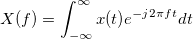
Commonly in engineering, “j” represents the imaginary value. “t” and “f” are real numbers representing time and frequency, respectively. In short, the FT decomposes the continuous temporal signal "x(t)" into a continuous complex function which changes with frequency. "x(t)" can be a song or a speech signal, which makes sense in the real world since any sound we hear is continuous and as time passes, it changes! The magnitude of "X(f)" is the visual equalizer!
However, considering the target platform is a discrete system ( i.e. a computer ), the signal’s frequent content is needed at regular intervals in time, not to mention the FT implies the ENTIRE signal x(t) is needed, the continuous FT cannot be computed precisely.
The implementation of the FT feasible for discrete systems is the Discrete FT ( DFT ), which can be found by discretizing the continuous variables in the original FT. The discretization can be done with the following expressions.
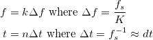
This process of discretizing continuous variables can be regarded as transformations in their own right; they both map their respective sets of real numbers ( “f” and “t” ) to natural numbers ( “k” and “n” ) by sampling. The “delta f” and “delta t” are commonly referred to as the frequency resolution and sampling period, respectively. “K” ( capital “k” ) is the number of possible frequencies from 0 to “fs-delta f”, inclusively. And, “fs” is the sampling rate. After performing the substitutions, the approximated FT has the following form.
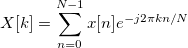
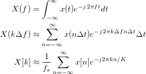 This approximated FT is further simplified down to the DFT by dropping the scalar, assuming the first sample starts at 0 and ends at “N-1”, and setting “K” to equal “N”. “N” indicates the total number of samples in the signal.
But, because each “X” needs to be computed for "k" ranging from 0 to “N-1”, a literal implementation of the DFT demands a lot resources due to its repetitiveness. Thus, the Fast FT ( FFT ) is employed virtually in any field related to signal processing to quickly generate the DFT’s result!
The most common FFT algorithm, and the one most relevant to the project, is the radix-2 Cooley-Turkey algorithm. Luckily, this is the one I am most familiar with ( again, it’s the most widely used )! So, after reviewing some of the details from Wikipedia, the algorithm can be concisely described as a “divide and conquer” algorithm that shortens computation time with a combination of reducing repeating operations, taking advantage of complex exponential identities, and recursively defining operations. This is my overly general definition, keep in mind!
The following summarizes how the algorithm can be expressed mathematically, which is computed for non-negative integers “k”, starting at 0 and ending at “N/2”.
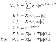
The powerful “divide and conquer” / recursive aspect of the algorithm is clear from the first three expressions! The first expression is simply the DFT, whereas the second and third expressions are the DFTs of the even and odd samples of the discrete signal "x[n]". But, how are those DFTs computed? Well, the same algorithm is applied recursively! In other words, the FFT can effectively be applied again and again for the terms “E[k]” and “O[k]”! And, in a FPGA, the structure of the Cooley-Turkey algorithm results in better performance per unit resource ( PPUR )! Just for the record, “performance” without any qualifiers refers to how fast the respective operation can complete, in this context.
Before I continue, I need to make an important observation regarding the performance of the DFT and the FFT! Notice I don’t directly say the FFT is faster than the DFT! In fact, I would actually argue the regular DFT is faster the FFT! The obvious rebuttal is “Andrew, even you pointed out the DFT has to complete more operations!” Another way of stating the same rebuttal is that the time complexity of the DFT is “O(N^2)”, whereas the FFT is “O(Nlog_2(N))”! The theoretical time complexities, however, only reflect sequential operations. That is to say, the time complexities assume nothing is parallelized. In theory, the DFT will finish in “O(1)” on a device capable of always parallelizing independent operations, whereas the FFT is limited to “O(log_2(N))” because recursion forces dependent operations. Because my target device is an FPGA, which is clearly capable of parallelizing independent operations, it has a very limited amount of resources ( i.e. logic, routing, and hard blocks ). And, since I already know the visual equalizer will need to perform the DFT over large data sets, FFT is the obvious choice!
Super cool! I think so, anyway! And, if you’ve made it this far in this explanation, you must ( or likely ) think this is super cool, as well!
Going back to the original problem of building a visual equalizer, there’s still the problem of how the FFT can be applied such that the DFT is generated “for each instance of time”. With the solution utilizing the bandpass filters, the visual equalizer can easily be updated for every new sample! Well, without jumping too much into the implementation, an update to the visual equalizer for every new sample would be wasteful. In fact, I think it’s very likely the FFT-solution has better performance per unit of power ( PPUP ) than that of the filter-solution, considering the latter would require many DSP operations running constantly ( not that I really considered the power constraints of this project ).
A monitor displays each frame of the visual equalizer. Thus, “for each instance of time” really means “for each frame with which the monitor is updated”. It is only necessary to perform the FFT once per frame! And, monitors don’t update fast when compared to the performance of the FFT!
There are still a bunch of problems that have yet to be addresses. However, those problems are what I like to refer to as “implementation problems”, which are addressed under implementation, of course. For now, the theory behind my visual equalizer’s implementation can be extended to update the latest video frame with the FFT of the latest set of audio samples!The Implementation: Making It Work!
At last, this discussion has finally reached the implementation, the fun and exciting part of the project! And, this, to me, is usually the most challenging part since “the theory” often lacks regard to real-world considerations. Of course, since I had already known a lot about my target hardware, I knew what changes to the theory I needed to make, ahead of time. More often than people would like, the theory in other projects would need to be revised due to real-world limitations ( e.g. money, size, energy, current technology, etc. ), hence all of engineering!
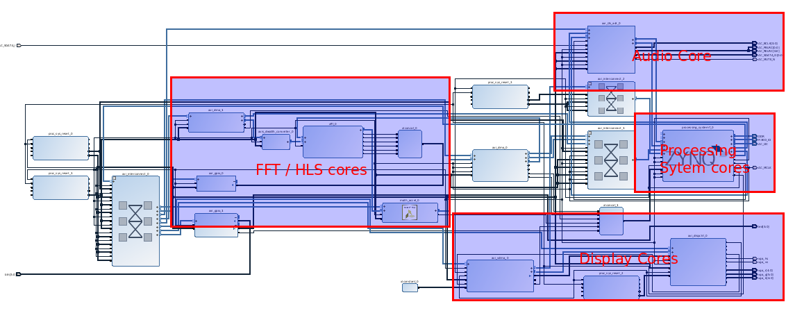
The figure above is a screenshot of a graphical representation of the RTL project, which was developed in Vivado 2016.2 IDE. The software, which executes on the MCP located in the “Processing System cores”, was all developed in the SDK, basically Eclipse. The target hardware is the Digilent Zybo board. As a way to organize this explanation, I divided the top module into fewer groups of components. For simplicity’s sake, I won’t discuss much detail on any of the “minor” cores. In this context “minor” refers to the cores that still contribute to the RTL design, but their roles are mainly to supplement the cores that perform the functions necessary to carry out the theory discussed earlier.
The “general flow”, how data moves through the RTL design, is the following. 24-bit audio samples are sampled by the “Audio Core” at approximately 48 kHz ( ~20.8 microseconds ). Those audio samples pass through the “Processing System cores” where CPU0, an ARM Cortex-A9 of the MCP, outputs those same audio samples back to the “Audio core”, and also buffers 16-bit versions of the audio samples. The “Audio Core” is a ADI AXI I2S controller which allows a host device to input or output PCM audio samples with the Zybo’s audio codec.
In order to ensure there are no delays, there are two buffers of size 1024, one for filling and the other for working. Once the filling buffer is filled, it becomes a working buffer and the original working buffer becomes a filling buffer. Once a filled buffer is ready, CPU0 initiates the 1024-point FFT operation with the Xilinx AXI FFT core ( ~63.820 microseconds ), located in “FFT / HLS cores”.
But, why did I chose to buffer 1024 audio samples and then perform the FFT? Well, the 1024 audio samples is my way of defining what “an instance of time” quantitatively means. With a ~48 kHz sample rate, 1024 audio samples indicates an “instance” is approximately 21.3 milliseconds or an update-rate of 46.9 Hz. Unfortunately, the FPS of my display is 60 Hz, but I decided to break that constraint for more samples in my FFT and for better frequency resolution. In a later version of this project, I will have to figure out a way to fix this particular issue!
Before the 32-bit complex samples ( 1.15Q imaginary and 1.15Q real ) are stored in a separate location in memory, a core created with High Level Synthesis ( HLS ) determines the magnitude of each audio sample. The FFT operation then alerts CPU1, another ARM Cortex-A9 in “Processing System cores”, upon completion.
The job of CPU1 is to generate the video frame. The frame itself is stored in memory from which the “Display Cores” reads in order to update the VGA interface. The main component of the “Display Cores” is the Digilent AXI Display core, I should point out. But, how is this frame generated in the first place? Well, the frame itself is divided into rectangles whose respective heights are varied according to the magnitudes. The different heights of each rectangle are indirectly computed from the magnitudes! The reasons for not just varying the heights directly from the 1024 magnitudes are all aesthetic reasons; I wanted the visual equalizer to look visually smooth and I wanted to be able to play around with the parameters of the visual equalizer, without having to re-compile ( synthesize / implementation ) the RTL project.
So, in order to achieve those conditions, I employed “two levels” of averaging. I’ll define this operation mathematically below.

“|X_1024[k,m]|” is of course the magnitude of the current FFT, where “each instance in time”, or 1024 samples, is referenced by the non-negative integer “m”. The “first level” of averaging is the “AVG_128” operation, which breaks the 1024 magnitudes down to 128 partitions and then averages each partition. The final result “X_128”, which I’ll call the “modified average”, is a weighted average among three different terms, the “second level” of averaging.
The first term weights the results of the “AVG_128” operation. The second and third terms are very similar. They both are weighted, previous results. But, the first is the previous partition during the same instance of time, whereas the second is the previous instance of time during the same partition. This second level of averaging is simply an Exponential Moving Average ( EMA ) filter! Super easy to implement, especially in an embedded application for which you want to avoid costlier filtration methods. However, the results are still very effective!
The different colors you see are a result of having the color of each pixel vary according to either where the partition’s respective rectangle is located on screen or the “modified average” of each partition!
That’s basically it!
One more thing! An attentive observer would notice my visual equalizer tends to look somewhat “triangular” compared to those commonly found. Specifically, the lowers frequencies tend to outweigh the higher frequencies! Well, there’s another “issue” with my implementation! I failed to take into consideration the majority of the an audio signal’s energy ( or any signal, really ) tends to be concentrated in the lower frequencies. My partitions are equally spaced, which wasn’t the best choice. What I should have done, and what I will do in the future, was create smaller partitions for lower frequencies but bigger partitions for higher frequencies!
NOW, that’s it!