I wanted to copy these figures from the Maxim application note, but they're copyrighted and whatnot, so I wrote some quick python to calculate Fourier transforms for piecewise-constant functions and drew my own.  I would have paid good money for access to something like this when I took those undergrad courses...

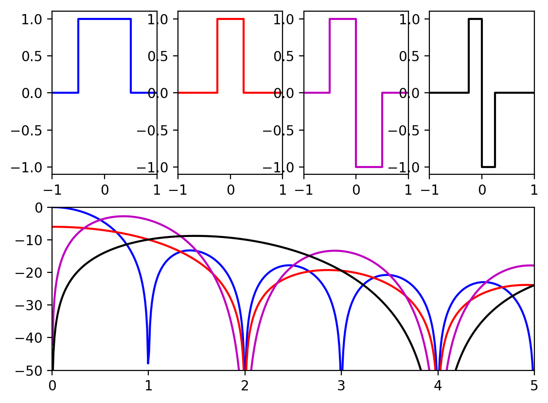
Along the top are the four DAC impulse responses supported in the MAX5879, and in the bottom plot are the corresponding output envelopes in dB vs frequency (1 = the sampling frequency, so the first Nyquist zone extends from 0 to 0.5). 

The first response (blue) is the familiar zero-order-hold, which just outputs a constant value during each sample period.  This is the response implemented in the FL2000 chip.  You can see that the output spectrum has zeros at multiples of the sampling frequency.

The second response (red) drops back to zero (known as return-to-zero) for half the sample period.  This results in an output envelope that has zeros at even multiples of the sampling frequency.  This is beginning to approach the ideal of an infinitely narrow output sample, which would have a flat output spectrum.

The third response (magenta) inverts the output for half the cycle.  This has a zero at DC, so is only useful for RF generation, not baseband signals, but has a higher envelope in certain Nyquist zones.

The last response (black) also inverts but returns to zero for half the period.

You can see how choosing one of these outputs from the DAC could really come in handy when using higher-order Nyquist zones: you can tailor the output envelope for the frequency you want to create.

One of the goals of this project is to create a simple, cheap add-on to the FL2k dongles to modify this response and allow better generation of higher frequencies.

Oh, I guess I'll drop the code that generates the figure here.  It's a one-off, so it ain't pretty, but it works:

#!/usr/bin/env python

import numpy as np
import matplotlib.pyplot as plt


t0 = np.array([-2, -1, -1, 1, 1, 2])*0.5
h0 = np.array([ 0,  0,  1, 1, 0, 0])

t1 = np.array([-4, -1, -1, 1, 1, 4])*0.25
h1 = np.array([ 0,  0,  1, 1, 0, 0])

t2 = np.array([-2, -1, -1, 0,  0,  1, 1, 2])*0.5
h2 = np.array([ 0,  0,  1, 1, -1, -1, 0, 0])

t3 = np.array([-4, -1, -1, 0,  0,  1, 1, 4])*0.25
h3 = np.array([ 0,  0,  1, 1, -1, -1, 0, 0])

fmax = 5
n_points = 1000

def plot_pair(t, h, style):
  f = np.linspace(-fmax, fmax, n_points)
  H = np.zeros(n_points, dtype=complex)

  # calculate Fourier transform H(f) for piecewise-constant function h(t)
  for i in range(1, len(t)):
    H -= h[i] * (np.exp(1j*2*np.pi*f*t[i])/(1j*2*np.pi*f) -
                 np.exp(1j*2*np.pi*f*t[i-1])/(1j*2*np.pi*f))


  plt.plot(t, h, style)
  plt.axis([-1, 1, -1.1, 1.1])
  plt.subplot(2, 1, 2)
  plt.plot(f, 20*np.log10(np.abs(H)), style)
  #plt.plot(f, np.square(np.abs(H)), style)

plt.subplot(2, 4, 1)
plot_pair(t0, h0, 'b')
plt.subplot(2, 4, 2)
plot_pair(t1, h1, 'r')
plt.subplot(2, 4, 3)
plot_pair(t2, h2, 'm')
plt.subplot(2, 4, 4)
plot_pair(t3, h3, 'k')
plt.axis([0, 5, -50, 0])
#plt.show()
plt.savefig('DAC_impulse_response.png', bbox_inches='tight', dpi=200)