 Alfonso Troya
Hi again!
We have some very good news, our Robot is moving!
The simulation environment is up and running. The calculations for the odometry and hardware integrations are done! There is still a lot to be developed, tested and integrated but we can say the first development milestone is complete and the Alfa version of the IMcoders closed.
DIFFERENTIAL DRIVE
To explain what is happening on the simulations we need first to explain with what kind of Robot we are dealing with. As this are the first tests we decided to keep it simple and go with a robot with differential drive. Don't you know what that means? No problem, here we have a small overview (information extracted from Wikipedia).
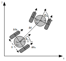
A differential wheeled robot is a mobile robot whose movement is based on two separately driven wheels placed on either side of the robot body. It can thus change its direction by varying the relative rate of rotation of its wheels and hence does not require an additional steering motion. If both the wheels are driven in the same direction and speed, the robot will go in a straight line. If both wheels are turned with equal speed in opposite directions, as is clear from the diagram shown, the robot will rotate about the central point of the axis. Otherwise, depending on the speed of rotation and its direction, the center of rotation may fall anywhere on the line defined by the two contact points of the tires.
ODOMETRY
Up this point everything is clear, isn't it? We have a robot with two wheels and based on the speed of them, the robot will change its direction and speed. The theory is clear, but... how can we calculate the movements of the robot?
To keep this entry short we are going to look at the calculations from a conceptual point of view, not going into detail in each step. We are planning an entry where all the concepts and maths involved in the calculations (Quaternions, rotations, sampling rate, etc..) will be covered in detail. Right now we need to finish all the things before the deadline for the [ROBOTICS MODULE CHALLENGE].
If you can't wait you can have a look at the code in our GIT repository, the maths and everything are there. Feel free to modify them and play around!
Odometry for differential drive robots is a really common topic and several algorithms to solve this problem can be easily found in the Internet (that is one of the reasons we decided to start with this kind of driving mechanisms). To perform these calculations, independently of the algorithm used, the calculation of the linear speed of the wheels are involve and that is exactly what we are going to do. Let's compare the calculations done when using traditional encoders and the needed ones with IMcoders to understand why the system works.
Traditional Encoders:
Traditional encoders are able to count "ticks" while the wheel is spinning, each "tick" is just a fraction of a rotation. Lets assume we have a robot with two wheels with 1 meter diameter each and one encoder in each wheel with 360 ticks per revolution (one rotation of one wheel clockwise implies a count of 360 ticks, and counterclockwise -360 ticks)
To calculate the linear velocity of one wheel we will ask the encoder its actual tick count. Lets assume the enconder answers with the tickcount 300. After 1 second we ask again and now the answer is 390. With this information we can now calculate the linear velocity of the wheel.
We know that in an arbitrary time (lets name it "t0") the tick count was 300 and one second later (lets call this time "t1") it was 390. Knowing that our encoder would count 360 ticks per revolution, an increase of 90 ticks implies a rotation of 90º. As duration between the two measurement is 1 second, we can easily calculate the linear speed of the wheel:

If we repeat the same procedure with the other wheel we can also calculate the linear velocity of the second wheel and use this information as input values for any already available differential drive odometry algorithm.
IMcoders:
With the IMcoders sensors the procedure is really similar, but the starting point is a little bit different. As you probably remember from our entry blog [REAL TESTS WITH SENSORS] the output of the sensor is the absolute orientation of the IMcoder in the space. That means that we can ask our sensor where is it facing in each moment.
To calculate the linear velocity of one wheel we will ask the IMcoder its actual orientation. Lets assume the sensor answers saying it is facing upwards (pointing to the sky +90º). After 1 second we ask again and now the answer is that it is facing forward (0º). With this information we can now calculate the linear velocity of the wheel.
We know in an arbitrary time (to keep the same naming lets name it also "t0") the initial orientation was 90º (sensor facing to the sky) and one second later (in time "t1") it was 0º (facing forward), clearly that is a 90º rotation in the orientation. As between the two measurement we waited 1 second, we can easily calculate the linear speed of the wheel.

If we repeat the same procedure with the other wheel we can also calculate the linear velocity of the second wheel and use this information as input values for any already available differential drive odometry algorithm.
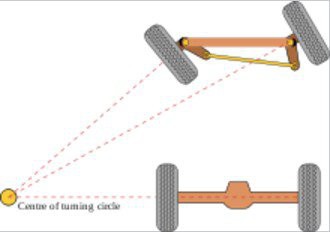
IMPORTANT: the output of the IMcoders sensor is the absolute orientation of the wheel in the space (3 axis; X, Y and Z), for all this calculations we are assuming the wheel is only spinning around one axis (which is the normal case for a robot with differential drive) but this is not the case for robots with ackerman steering, where this tridimensional orientation can be really helpful as the wheel change its position in two diferent axis:
SIMULATION
Ok, ok, theory is good and it "should" work, but... does it really work? Of course!
To understand what is really happening in the simulation let's split the system to explain what are we looking at. The system works as follow:
- Movement commands are being sent to a robot model in a simulation environment (Gazebo) where two of our IMcoders are attached to the wheels of the robot model (one per wheel).
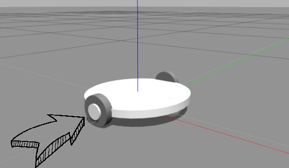
- When the robot moves, the attached IMcoders sent the actual orientation of the wheels to our processing node.
- The node outputs odometry message (red arrow) and a transformation to another robot model which we display in a visualization tool called rviz.
- The robot moves based on this odometry information!
Now that our simulation environment is working we can characterize our system, there are several questions still open this simulation model will help us to solve.
- How fast can a wheel spin and be measure by our IMcoders?
- How many bits do we need in the Accelerometer/Gyros in the IMcoders to produce a reliable odometry?
- Which algorithm performs better in different scenarios?
- etc...
Discussions
Become a Hackaday.io Member
Create an account to leave a comment. Already have an account? Log In.