The next step in designing my "most complicated freezer closed loop control system" was to create a linear observer.
For my system model I have three temperatures I am currently measuring and I want to get rid of the temperature probe that measures the sidewall of the freezer! Why, you might ask, would you go through this extra complicated step and decrease the reliability of your system by increasing complexity?
1.) Because I can.
2.) So I can learn.
Just to point this out: One of my coworkers built a kegerator recently. He purchased a ~$60 box that hangs on his wall that his freezer plugs into and has a temperature probe that he can stick either in a carboy or next to one of his kegs to control the temperature of the freezer. It most likely uses some simple PID control algorithm. I just want to put that out there so that everyone realizes the ridiculous level of complexity I am adding into what could be a very simple control system…
With that out of the way, the two textbooks I am referencing are:
Feedback Control Systems (Franklin, Powell), fourth edition
Control System Design, An introduction to State-Space Methods (Friedland), First Edition
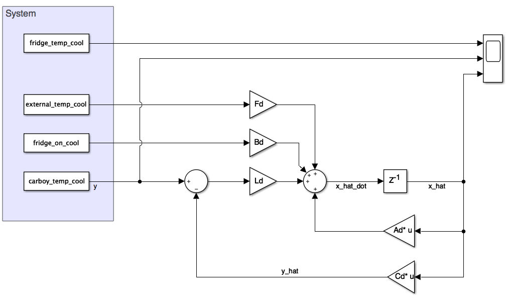
I designed my linear observer using the example 7A in Friedland. (See page 264 if interested.) Chapter 7 in Franklin also helped as well. I attached my math as a design file named “Linear Observer Design Sept 9 2018.pdf for those who are interested in taking a quick review.
I then proceeded back to Matlab and Simulink to see if my observer actually worked.
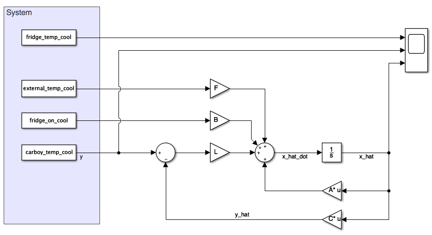
The first step was to validate operation in the continuous time domain. I setup a quick model. See below.
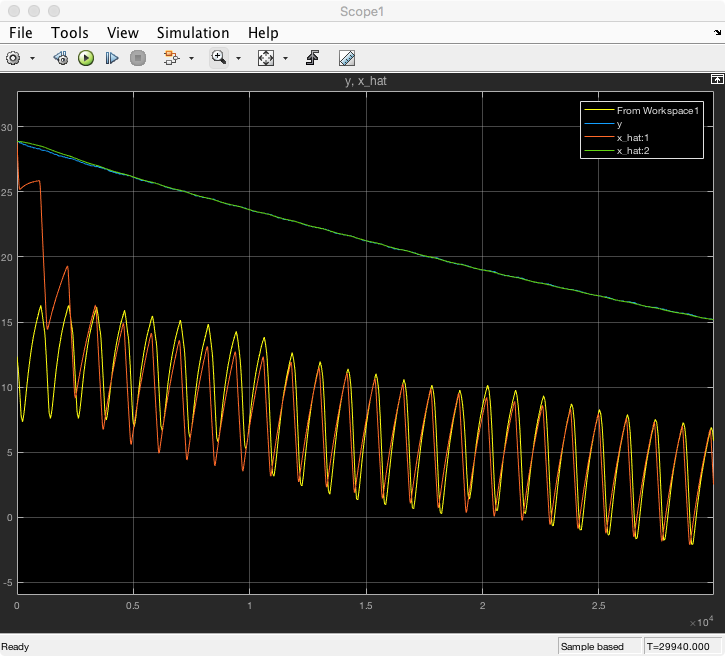
The simulation results tuned beautifully when I placed the two closed loop poles at 0.001 rad/s.
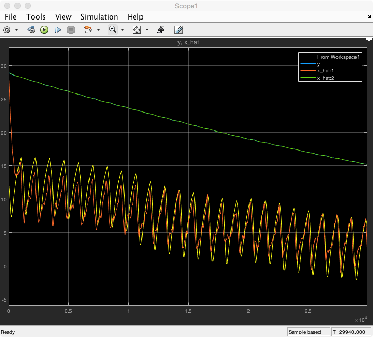
However as I moved the two poles further into the right half plane (i.e. faster response) the estimated value for the freezer wall would converge fast but started to have noticeable noise. See below fora plot with poles at 0.005 rad/s.
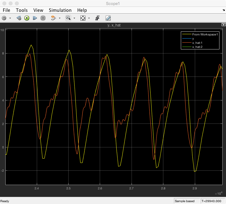
Close up image below.
For initial system design I selected a pole at 0.001 rad/s. I then converted by continuous time model into the digital domain. I selected a sampling time of 1 second. Matlab has a nice “c2d” function that I avoided. I ended up quickly coding the conversion algorithm documented in chapter 8 (pg. 676) in Franklin and using c2d to check my work. I then setup a new simulink model to validate that I didn’t mess anything up. The simulink model is below. It gave exactly the same results as the continuous time model.
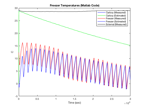
I then wrote the code for the state space algorithm in Matlab. I did this so that I could quickly plot the results of the coded algorithm prior to coding them into the teensy controller. I am glad I did as I quickly caught some typo errors that would have had me scratching my head. As you will also notice it takes approximately 30 to 60 minutes for the freezer wall temperature estimate to converge to the measured value. This is a LOT of time between troubleshooting. Code is below for those interested.
% ----- Digital Code Verification -----
t = 0:Ts:time_cool(end);
Te = my_interp(external_temp_cool,t);
Tc = my_interp(carboy_temp_cool,t);
Tf = my_interp(fridge_temp_cool,t);
fridge_on = my_interp(fridge_on_cool,t);

Tc_e = zeros(size(t));
Tf_e = zeros(size(t));
%Tc_e(1) = Te(1);
%Tf_e(1) = Te(1);

for loop = 1:(length(t)-1)
    [Tf_e(loop+1), Tc_e(loop+1)] = observer_algorithm(Ad,Bd,Fd,Ld,Tf_e(loop),Tc_e(loop),Tc(loop+1),fridge_on(loop+1),Te(loop+1));
end

plot(t,Tc,'b');
hold on
plot(t,Tc_e,'g');
plot(t,Tf,'r');
plot(t,Tf_e,'b');
plot(t,Te,'k');
title('Freezer Temperatures (Matlab Code)');
legend('Carboy (Measured)','Carboy (Estimated)','Freezer (Measured)','Freezer (Estimated)','External (Measured)');
xlabel('Time (sec)');
ylabel('C');
hold off
The function "observer algorithm" is below.
function [Tf_e, Tc_e] = observer_algorithm(Ad, Bd, Fd, Ld, Tf_e_old, Tc_e_old, Tc, fridge_on, Te)
    a_11 = Ad(1,1); % A Matrix          0.9938
    a_12 = Ad(1,2); %                   0.0044
    a_21 = Ad(2,1); %                   0.0003067
    a_22 = Ad(2,2); %                   0.9997
    b = Bd(1);      % B Matrix          -0.4272
    f = Fd(1);      % F Matrix          0.0018
    l_Tf = Ld(2);   % Gain Matrix       0.0094
    l_Tc = Ld(1);   % Gain Matrix       0.6245

    error = Tc - Tc_e_old;

    Tf_e = Te*f + b*fridge_on + l_Tf*error + Tf_e_old*a_11 + Tc_e_old*a_12;
    Tc_e = l_Tc*error + Tf_e_old*a_21 + Tc_e_old*a_22;
end
I posted the code because originally when I started designing controller algorithms in my spare time (yes, this is my hobby!) I had no idea on how to actually write the code for a digital controller. It took me several weekends of staring at text books before it "clicked". I wanted to share above as going from block diagrams you see in textbooks to the actual code to implement the algorithm is NOT obvious. Or at least it wasn't to me.
The next step was to implement the linear observer in the teensy. I quickly found out that 1 sample a second for my interrupt was optimistic! I currently have the teensy, reading the digital temperature sensors, computing the weight of the scale, performing calculations for the linear observer and then printing all the changing variables out over serial to the Raspberry Pi during each interrupt function. This takes anywhere up to 2-3 seconds. The two slowest parts of the interrupt are reading the digital temperature sensors and the serial communication to the Pi. It is very easy to optimize this code. Realistically an interrupt should NOT be used for performing serial communication however I previously had the interrupt running every 60 seconds when I was recording data to model the system and there was plenty of time for serial communication.
To keep the project moving I elected to change the sampling period to 10 seconds. This is still wildly fast for the speeds at which the system dynamics in my freezer should be changing and allows me to send all the outputs from the calculations of the observer (and soon to come control algorithm) to the Pi so that I can troubleshoot the algorithms.
Based on the output of the linear observer results in Matlab code (not simulink) I increased the system poles to 0.005 rad/s. I believe the reason that Simulink is having issues at 0.005 rad/s is that the signals I am using to validate the observer were sampled at a 60 second interval. To increase the resolution for the simulink algorithms there is interpolation occurring that creates noise that is throwing off the simulation. See below for the output from the Matlab code with poles at 0.005 rad/s.
Also interesting is that the Matlab code implementing my linear observer shows the linear observer goes unstable if I increase the closed loop observer poles much beyond 0.005 rad/s. I believe this is due to the fact that I am only sampling every 10 seconds. The closed loop bandwidth of 0.005 rad/s is ~0.0008 Hz. This is about ~100 times slower than my sampling rate. As my poles move right I am getting close to that magic point where the digital sampling rate is less than 20 times the closed loop bandwidth (i.e. 0.005 Hz). At this point all bets are off and the system can be unstable simply because you are not sampling fast enough to approximate continuous control anymore. Also there is noise in the sampling due to the digitization of the temperature samples. While I know this noise is present I haven’t tried to really come to grips with how sensor noise is impacting my algorithm. It could be impacting me more than I am aware.
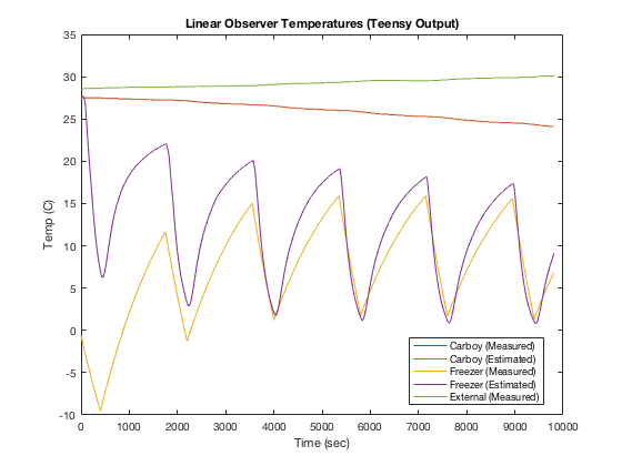
Anyway, it works! See below for a plot of my estimator converging with the measured freezer temperature. This is a plot of the output directly from the teensy. (Matlab was only used to read in the values saved by the Raspberry Pi and plot the results.) The estimate for the Carboy temperature converges very quickly. The estimate for the freezer temperature, in this case, took about an hour. Each cycle, where it cools and then warms is about 30 minutes. The freezer is on for 25% of the 30 minutes.
Stay tuned. Next is closing the loop on controlling the freezer. Whoo hoo! :-)
Discussions
Become a Hackaday.io Member
Create an account to leave a comment. Already have an account? Log In.