PART 1
The optical encoder’s disc is made of glass or plastic with transparent and opaque areas. A light source and photodetector array read the optical pattern which results in a square wave signal. The rising and/or falling edge of the sensor square wave output can be used to count (each count is known as a ‘tick’) and estimate the distance traveled by a wheel. Incremental encoders can be hooked to the interrupt pins of the Arduino board to trigger every tick. Gyroscopes are sensors used to obtain the orientation of a body on a particular plane or in space. Yaw rate gyroscopes are sensors that give the rate of change of angular position of a body in a particular axis. Such sensors can be used to determine the angular position of a moving body. These two sensors can be used in conjunction to estimate the state of the robot.
Odometry is the use of data from moving sensors (wheel encoders) to estimate a change in position over time. Odometry is used by some robots, whether they are legged or wheeled, to estimate their position relative to a starting location. This method is sensitive to errors. Rapid and accurate data collection is required for odometry to be used effectively. Odometry can be implemented on a differential drive robot with two sets of wheel encoders on either shaft of the motor attached to a wheel.
Let the radius of the wheel be R.
Let y and z be the number of counts or ‘ticks’ from the encoder.
Let Nl and Nr be the counts or ‘ticks’ per each revolution of the wheel.
Dl = 2 × π × R × (y/Nl) (1)
Dr = 2 × π × R × (z/Nr) (2)
Dc = (Dl + Dr) / 2 (3)
Equation (1) and (2) represent the distance traveled by each wheel. Equation (3) represents the distance traveled by the robot.
Φ= (180 / π) × (Dl – Dr) / L (4)
Equation (4) represents the current angle of the differential drive robot, where L is the wheelbase (distance between the two wheels of the robot). Equations (1), (2), (3) & (4) are used to estimate the current position of the bot.
Xpos = Dc × (180/π) × sin(Φ) (5)
Ypos = Dc × (180/π) × cos(Φ) (6)
Equation (5) and (6) give the current position of the bot along the x-axis and y-axis. Hence these equations determine the position of the bot in the Cartesian coordinate form.
Having the current position and the orientation of the robot it is possible to control and navigate the robot through a series of coordinates. PID algorithm can be used to navigate the robot, where the control variable is the angle of the bot (Φ), the process variable is the desired angle (Φd) and the manipulated variable is given to the motors of the differential drive robot.
Φd = (180 / π) × arctan((Yg-Ypos) / (Xg-Xpos)) (7)
Equation (7) can be used to generate the desired angle of the robot. The desired angle is the formed by the line joining the current position coordinate of the robot to its destination
PART B
One essential computation for robots for autonomous navigation is path planning. There are three basic path planning algorithms available namely A star, Dijkstra's and Gradient Descent.
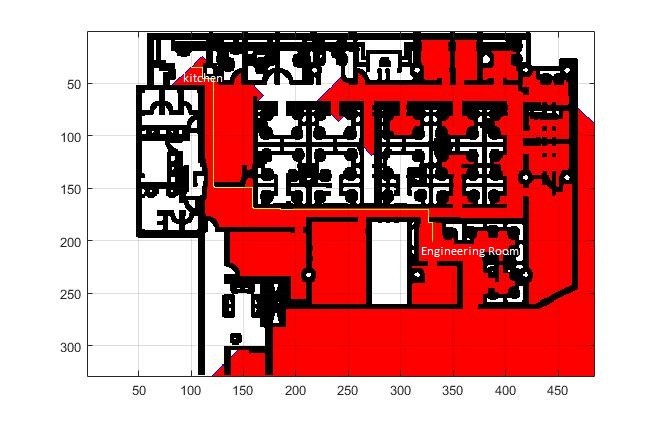
Dijkstra’s is an algorithm for finding the shortest path between nodes in a graph, which may represent, for example, road networks. The algorithm basically associates a cost on every node it searches from start to goal position. It also keeps a track of the parent positions to form a route at the end of the algorithm. If the nodes around the current node is a free space and not an obstacle or not already searched for it add it to a list of nodes to be checked in the following iterations. In the following iteration, it only chooses the node with the minimum cost. The cost of a node is determined by its distance from the start position. The loop breaks when it hits the goal position. There are a lot more technicalities in the algorithm. You can go through the MATLAB code below to get a better idea of its implementation.
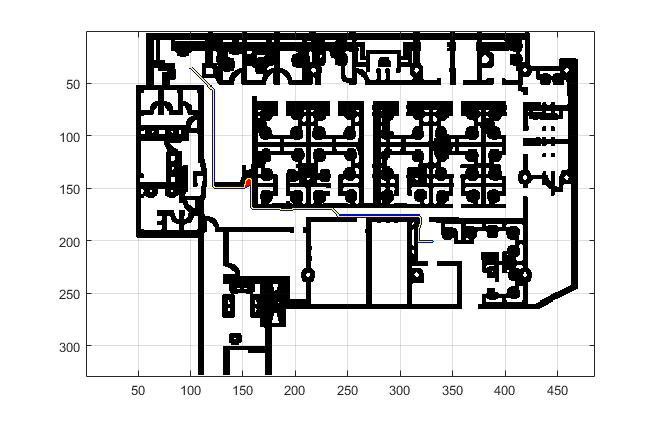
The A star at its crux is very similar to Dijkstra’s algorithm, but the costs are assigned very differently. Each node gets a cost on its euclidian distance from the goal node. This Heuristic helps the algorithm select nodes in that are closer to the goal rather than just looking for the one with the lowest cost. The result of which enables the algorithm search only in the direction of the goal node.
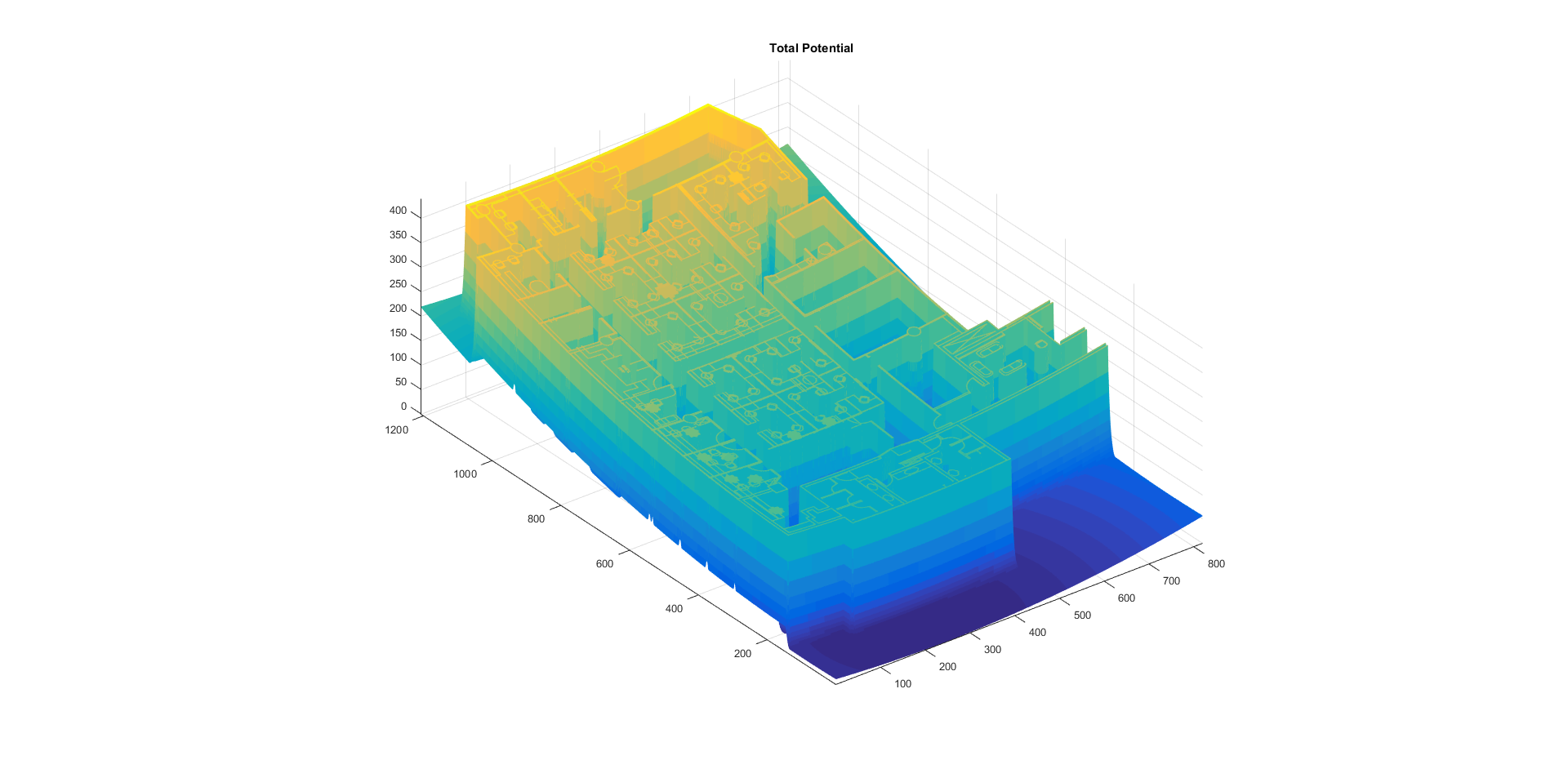
The third method involves Gradient Descent and repulsive and attractive potential fields. In layman’s terms, it’s like manipulating the map into the pinball game where the ball avoids the obstacles and moves in the direction of the gradient. This method can be used to create smooth trajectories unlike A* and Dijkstra’s and is computationally more expensive.