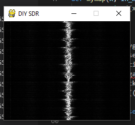
• Live waterfall

    Max-Felix Müller05/11/2019 at 23:03 0 comments

    After some fiddeling around with pygame.image I got this to work.

    I use pygame because I though I knew how to display an iamge there. It turns out I didn't. Well at least now I guess I do.

    Later on I will propably switch to a different gui library. I'm thinking of Tkinter.

    And here is the code:
    from matplotlib import mlab as mlab
    from rtlsdr import RtlSdr
    import numpy as np
    from PIL import Image
    import time
    import pygame
    
    DISPLAY_WIDTH = 256
    DISPLAY_HEIGHT = 200
    
    sdr = RtlSdr()
    # configure device
    sdr.sample_rate = 2.4e6  # Hz
    sdr.center_freq = 94.7e6  # Hz
    sdr.freq_correction = 60   # PPM
    sdr.gain = 'auto'
    
    
    image = []
    
    
    def get_data():
        samples = sdr.read_samples(16*1024)
        power, _ = mlab.psd(samples, NFFT=1024, Fs=sdr.sample_rate /
                            1e6)
    
        max_pow = 0
        min_pow = 10
    
        # search whole data set for maximum and minimum value
        for dat in power:
            if dat > max_pow:
                max_pow = dat
            elif dat < min_pow:
                min_pow = dat
    
        # update image data
        imagelist = []
        for dat in power:
            imagelist.append(mymap(dat, min_pow, max_pow, 0, 255))
        image.append(imagelist[round(len(
            imagelist)/2)-round(len(imagelist)/8): round(len(imagelist)/2)+round(len(imagelist)/8)])
        if len(image) > 200:
            image.pop(0)
    
    
    def mymap(x, in_min, in_max, out_min, out_max):
        return int((x - in_min) * (out_max - out_min) / (in_max - in_min) + out_min)
    
    
    pygame.init()
    gameDisplay = pygame.display.set_mode((DISPLAY_WIDTH, DISPLAY_HEIGHT))
    pygame.display.set_caption(f"DIY SDR")
    clock = pygame.time.Clock()
    background = pygame.Surface(gameDisplay.get_size())
    background = background.convert()
    background.fill((0, 0, 0))
    
    game_quit = False
    
    while not game_quit:
    
        gameDisplay.blit(background, (0, 0))
    
        for event in pygame.event.get():
            if event.type == pygame.QUIT:
                game_quit = True
    
        get_data()
        outimage = np.array(image, np.ubyte)
        outimage = Image.fromarray(outimage, mode='L')
        outimage = outimage.convert('RGBA')
        strFormat = 'RGBA'
        raw_str = outimage.tobytes("raw", strFormat)
        surface = pygame.image.fromstring(raw_str, outimage.size, 'RGBA')
        gameDisplay.blit(surface, (0, 0))
        pygame.display.update()
        clock.tick(60)
    
    pygame.quit()
    
    try:
        pass
    except KeyboardInterrupt:
        pass
    finally:
        sdr.close()

  • Welcome Maurice

    Max-Felix Müller05/10/2019 at 19:46 0 comments

    Welcome Maurice to the project team!

    Maurice is a friend of mine who also studies electrical engineering. He too wants to learn about Python and DSP, as well as SDR.

  • Waterfall

    Max-Felix Müller05/10/2019 at 19:43 0 comments

    Next up: I want to create a waterfall showing the power distribution over the recorded bandwidth over time.

    To do so, I save all the spectrums I calculate in one array. The it is as simple as putting that array in a file.

    imagelist = []
        for arr in image:
            thislist = []
            for dat in arr:
                #dat = 10 * math.log10(dat)
                thislist.append(mymap(dat, min_pow, max_pow, 0, 255))
            imagelist.append(thislist)
        largearray = np.array(imagelist, np.ubyte)
    
        im = Image.fromarray(largearray, mode='L')
        im.save("ichbineinwasserfall.bmp")

    My main problem was, that I didn't set the data type of the numpy array so the conversion with pillow into an image as a byte array failed.

    This is the result for 94.7MHz. The spectrum is shown in a lot of other images I uploaded so I don't want to post it yet again.

    By the way: I use 94.7 as center frequency mostly because there is a radio station near me so I have a good signal to practice with 24/7. 

    The next step is to combine the waterfall and the graph in one window.

  • Fixing the large spectrum

    Max-Felix Müller05/08/2019 at 15:23 1 comment

    It came to my mind that it's possible that the chip I use can/does not update it's center frequency during operation.

    So I edited the code to reinitialize the device completly for each step in the for-loop.

    Here is the new loop:

    for i in np.arange(50, 1000, SAMPLERATE/1e6):
        sdr = RtlSdr()
    
        # configure device
        sdr.sample_rate = SAMPLERATE
        sdr.center_freq = i*1e6  # Hz
        sdr.freq_correction = 60   # PPM
        sdr.gain = 'auto'  # 4
        samples = sdr.read_samples(8*1024)
        sdr.close()
        sdr = None
        # use matplotlib to estimate and plot the PSD
        power, psd_freq = mlab.psd(samples, NFFT=1024, Fs=SAMPLERATE /
                                   1e6)
        psd_freq = psd_freq + i
        powe = np.concatenate((powe, np.array(power)))
        freq = np.concatenate((freq, np.array(psd_freq)))
        print(f"{i}/1000")

    The print statement at the end is just to keep track of how long it's going to take. This bit ran for about 7 minutes, because it is very slow to reinitialize like this all the time. There has to be a better way...

    I'll keep searching for that. During that time you can enjoy the new output:

  • Something seems off...

    Max-Felix Müller05/07/2019 at 18:32 0 comments

    ...and I can't quite explain it.

    During my testing I finally managed to have the broad spectrum from earlier all as one continuous array (so the plot consists of one line only, so to speak). Running it over a range from 50MHz to 1Ghz I expedcted to see a range where my antenna picks up better signals since it iss in tune, but instead it all looks the same:

    That's the full range I recorded.

    And here it is zoomed in at a random position.

    Notice the repeating pattern?

    My first suspicion was, that the center frequency is alwayys at the peak (which is actually true here). But when I ran the "live plot" code and moved the center frequency there the peaks stayed at their frequencies.

    Here's another picture of that:

    Notice that in this case, it is not the center frequency having the peak value.

    Here the code I used to put the measurements in one array. Maybe there's a mistake I'm not aware of?

    powe = np.ndarray(0)
    freq = np.ndarray(0)
    
    for i in np.arange(50, 1000, sdr.sample_rate/1e6):
        sdr.center_freq = i*1e6  # Hz
        samples = sdr.read_samples(8*1024)
        # use matplotlib to estimate and plot the PSD
        power, psd_freq = mlab.psd(samples, NFFT=1024, Fs=sdr.sample_rate /
                                   1e6)
        psd_freq = psd_freq + sdr.center_freq/1e6
        powe = np.concatenate((powe, np.array(power)))
        freq = np.concatenate((freq, np.array(psd_freq)))

    During my testing I also figured out what the sample rate I can set is actually about. It is the frequency span which is sampled. As an example setting it to 2.4Mhz (standard) and the center frequency to 94Mhz, the recorded data will be in the range 94Mhz +/- 1.2MHz. The limits I can set the sampling rate to are 1Mhz up to 3.2Mhz. 

  • Timing the loop

    Max-Felix Müller05/07/2019 at 12:25 0 comments

    I want to find out what takes so long in my loop. So I made some measurements to time different parts.

    Here are the results for the settings in the previously uploaded code:

    Timings (over 210 cycles):
    Sampling: 62.0748690196446
    Math: 34.39687547229585
    Plotting: 6.701296851748512

    The times shown here are in milliseconds.

    The code was configured to take n = 128*1024 samples for each plot. With a sample rate fs = 2.4Msps we can calculate:

    ts = 1/fs

    t = n * ts = 54ms

    Which is close enough.

    By reducing the number of samples to n = 64*1024 the time it takes to collect them also gets cut in half. Furthermore the time the program takes to calculate the fft is only about a third:

    Timings (over 62 cycles):
    Sampling: 28.427654697049046
    Math: 10.655737692309964
    Plotting: 4.603389770753922

    Again, the times are in ms.

    How far can we go?

    To calculate the fft I set the number of slots to 1024. So technically down to 1024 samples the times will decrease. Going even lower will force the psd function to fill missing values with zeros. This is called zero-padding. My limited testing had it seem like the time it takes to calculate the fft would go up when zero-padding starts. Sampling time obviously decreases further.

    These times are for 1024 samples:

    Timings (over 78 cycles):
    Sampling: 0.28314040257380557
    Math: 0.1401809545663687
    Plotting: 3.5302119377331853

    Where's the downside to decreasing the number of samples?

    Have a look for yourself:

    The first picture shows one reading of 128*1024 samples while the second picture only took 1024 samples.

    Notice that you can still clearly see the peaks in the signal.

    So what sampling rate shall I choose? I have no idea. Further testing has to be made. I guess it depends on what I am trying to accomplish witth the collected data.

  • Larger plot

    Max-Felix Müller05/05/2019 at 21:20 0 comments

    As you may have noticed, the data I read in is very focused around the center frequeny.

    Here is my first attempt to plot a broader spectrum.

    from rtlsdr import RtlSdr
    import matplotlib.pyplot as plt
    import numpy as np
    
    sdr = RtlSdr()
    
    # configure device
    sdr.sample_rate = 2.4e6  # Hz
    # sdr.center_freq = 94.7e6  # Hz
    sdr.freq_correction = 60   # PPM
    sdr.gain = 'auto'
    
    for i in range(70, 130, 2):
        sdr.center_freq = i*1e6  # Hz
        samples = sdr.read_samples(256*1024)
        # use matplotlib to estimate and plot the PSD
        plt.psd(samples, NFFT=1024, Fs=sdr.sample_rate/1e6, Fc=sdr.center_freq/1e6)
    
    sdr.close()
    
    plt.xlabel('Frequency (MHz)')
    plt.ylabel('Relative power (dB)')
    plt.show()

     The center frequency is increased in small steps. For every step, the output is caculated and added to the graph. Ideally I want to combine all samples into one plot (same color, continuos values) but today there's no time left.

    Another thing is the automatic gain which might throw off measurements taken at different times, I will check that out.

    PS: Yes, it is. I set the gain to always be 4 for now.

  • First live data

    Max-Felix Müller05/05/2019 at 21:15 0 comments

    The demo code only shows raw sample data. There is also another demo that converts the samples into a plot, showing the frequency and power.


    But I wanted more. Why not have that plot updated as new samples come in?

    I recently learned about the matplotlib animation thingy, which enables you to update your graph at a given itnerval.

    I haven't quite figured out how to run it as a complete seperate thread so while the window is opened, the program doesn't continue, but at least it updates.

    So here's my code:

    from matplotlib import pyplot as plt
    import matplotlib.animation as animation
    from rtlsdr import RtlSdr
    import numpy as np
    
    sdr = RtlSdr()
    # configure device
    sdr.sample_rate = 2.4e6  # Hz
    sdr.center_freq = 94.7e6  # Hz
    sdr.freq_correction = 60   # PPM
    sdr.gain = 'auto'
    
    fig = plt.figure()
    graph_out = fig.add_subplot(1, 1, 1)
    
    
    def animate(i):
        graph_out.clear()
        #samples = sdr.read_samples(256*1024)
        samples = sdr.read_samples(128*1024)
        # use matplotlib to estimate and plot the PSD
        graph_out.psd(samples, NFFT=1024, Fs=sdr.sample_rate /
                      1e6, Fc=sdr.center_freq/1e6)
        #graph_out.xlabel('Frequency (MHz)')
        #graph_out.ylabel('Relative power (dB)')
    
    
    try:
        ani = animation.FuncAnimation(fig, animate, interval=10)
        plt.show()
    except KeyboardInterrupt:
        pass
    finally:
        sdr.close() 

    While the window is open, every 10ms (or slower if the calculations take too long, which they do), new samples will be collected. Matplotlib provides a function called psd() which automatically plots power over frequency and adjusts for the center frequency as well as the sampling frequency.

    But what if I want to contine further with the power and frequency data?

    For example, if I want to output the common waterfall, I would need the power and freuqency values as a list or an array. Numpy array would be preferred but whatever works is ok for now.

    Well I did some googling and found this:

    # new import
    from matplotlib import mlab as mlab
    
    # new plot
    power, psd_freq = mlab.psd(samples, NFFT=1024, Fs=sdr.sample_rate /
                                   1e6)
        psd_freq = psd_freq + sdr.center_freq/1e6
        graph_out.semilogy(psd_freq, power)

     The formating got a bit lost there but you get the gist of it I guess.

    This way, the psd function returns the values instead of directly plotting them. The only thing left to do is to shift the results to the previously set center frequency.

    Notice that the frequency shown is in MHz.

  • Setting it all up

    Max-Felix Müller05/05/2019 at 21:02 0 comments

    I use VS Code as my programming enviorment for Python.

    As radio I used the Nooelec NESDR Smartee, which was the cheapest one I found that looked usefull when I bought it. It also comes with different antennas and has a SMA connector which is a plus for me.

    My only complaint is that it has a limited band but for that price I can live with it. I don't yet want to invest in a Hack RF One.

    You will need the pyrtlsdr module to easily interface with your radio. That in turn depends on librtlsdr being installed. You can download both from the links I provided in this project.

    To enable Python to interact with your radio, extract all the files from librtlsdr directly into your Python folder.

    Example: "D:/Programme/Python"

    Now you should be able to run the demo code from pyrtlsdr.

    I copy pasted it here for completion, but I do not claim any rights here.

    from rtlsdr import RtlSdr
    
    sdr = RtlSdr()
    
    # configure device
    sdr.sample_rate = 2.048e6  # Hz
    sdr.center_freq = 70e6     # Hz
    sdr.freq_correction = 60   # PPM
    sdr.gain = 'auto'
    
    print(sdr.read_samples(512)) 

    Source