 MS-BOSS
General parameters
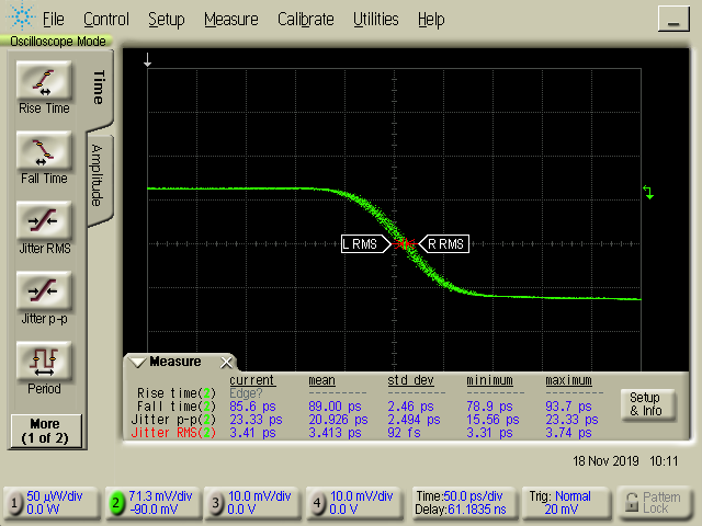
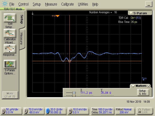
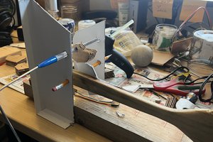
The reflectometer is able to measure in 20 ps steps (or any other step, it is just a matter of software configuration). The pulse generator makes rectangular wave with risetime of 85 ps. Measured risetime is about 200 ps. As a standalone device, it can detect simple discontinuities, such as shorts, disconnected cable, a split which halves impedance. When connected to PC, it can perform OSL calibration and show calibrated data.
If you want to know more, look into project logs.
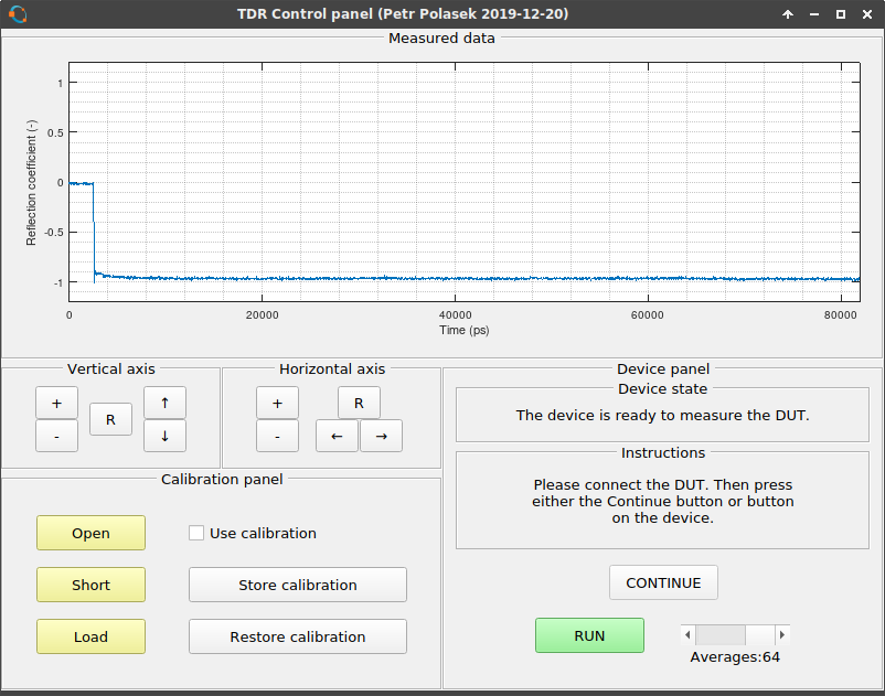
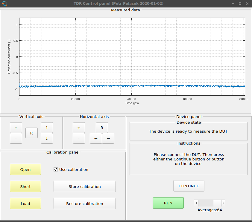
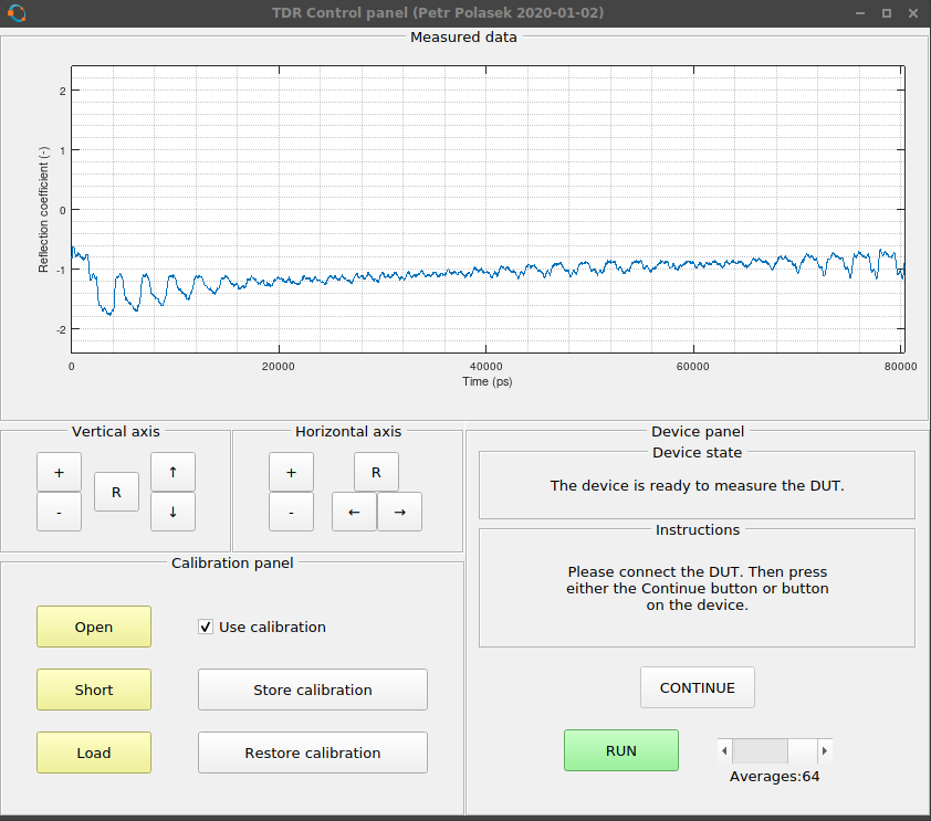
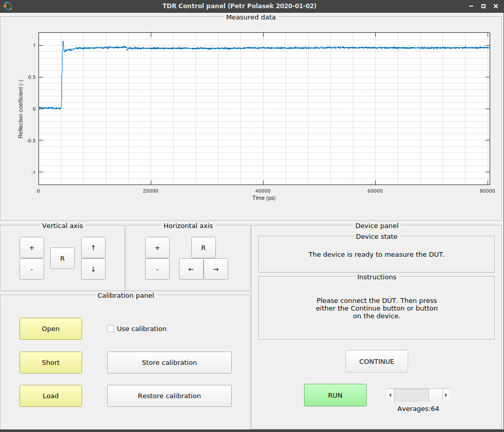
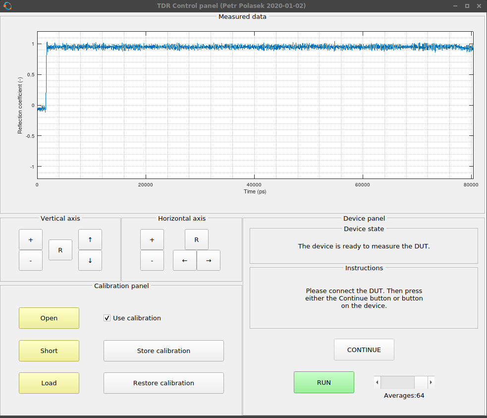
GUI in Octave
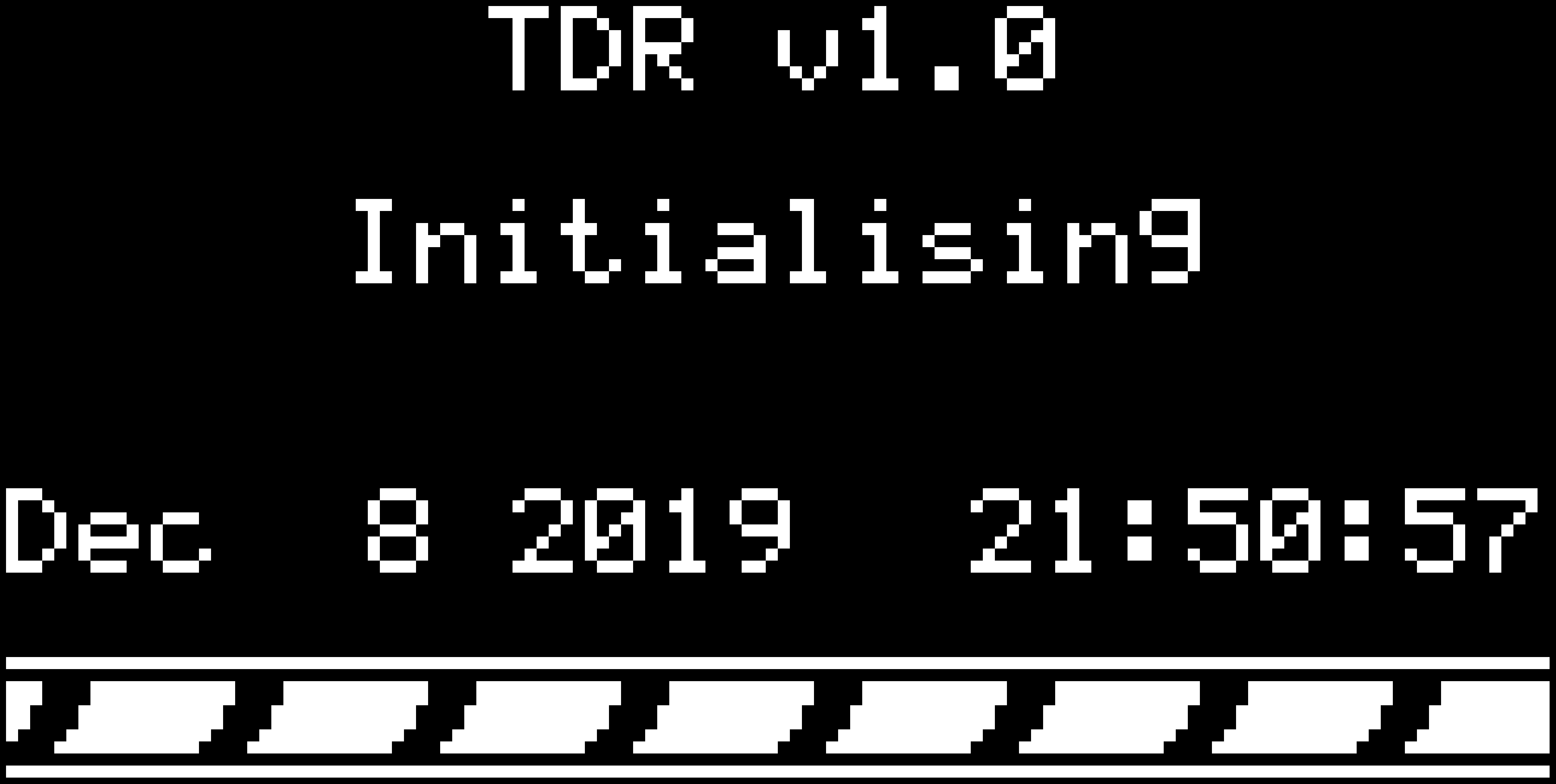
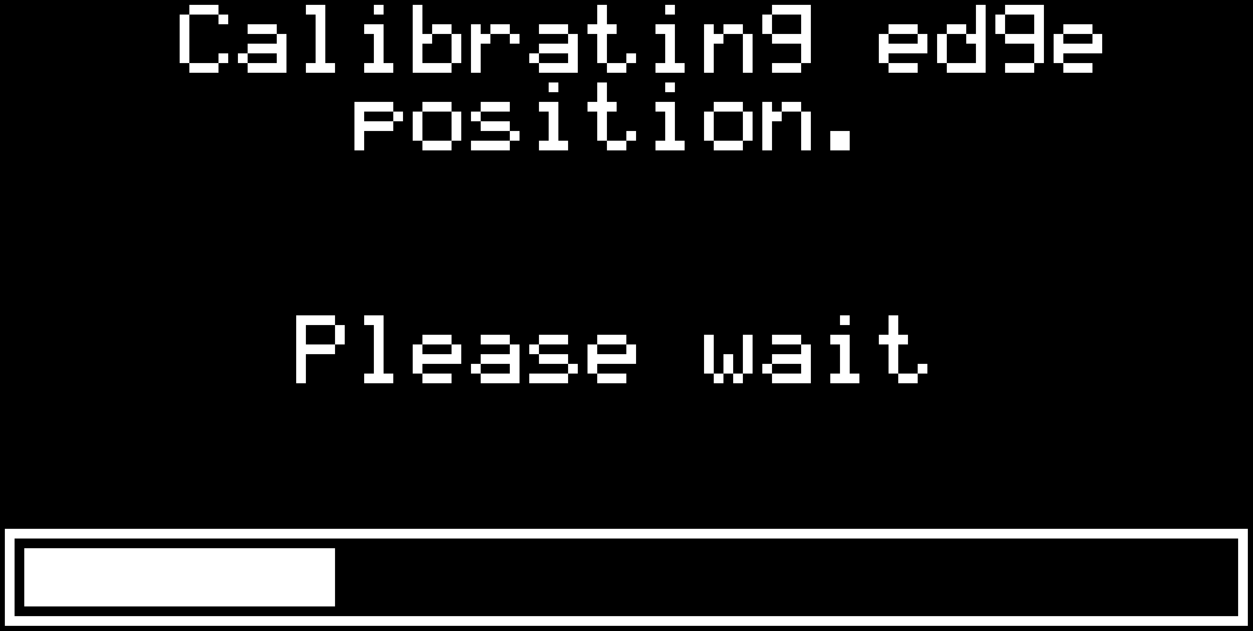
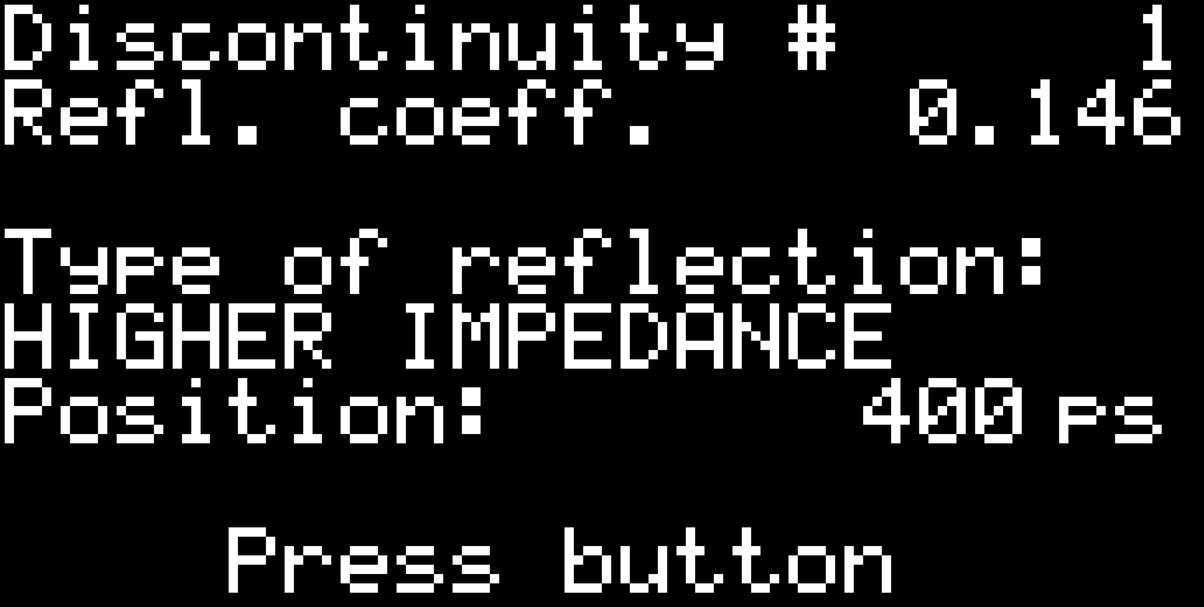
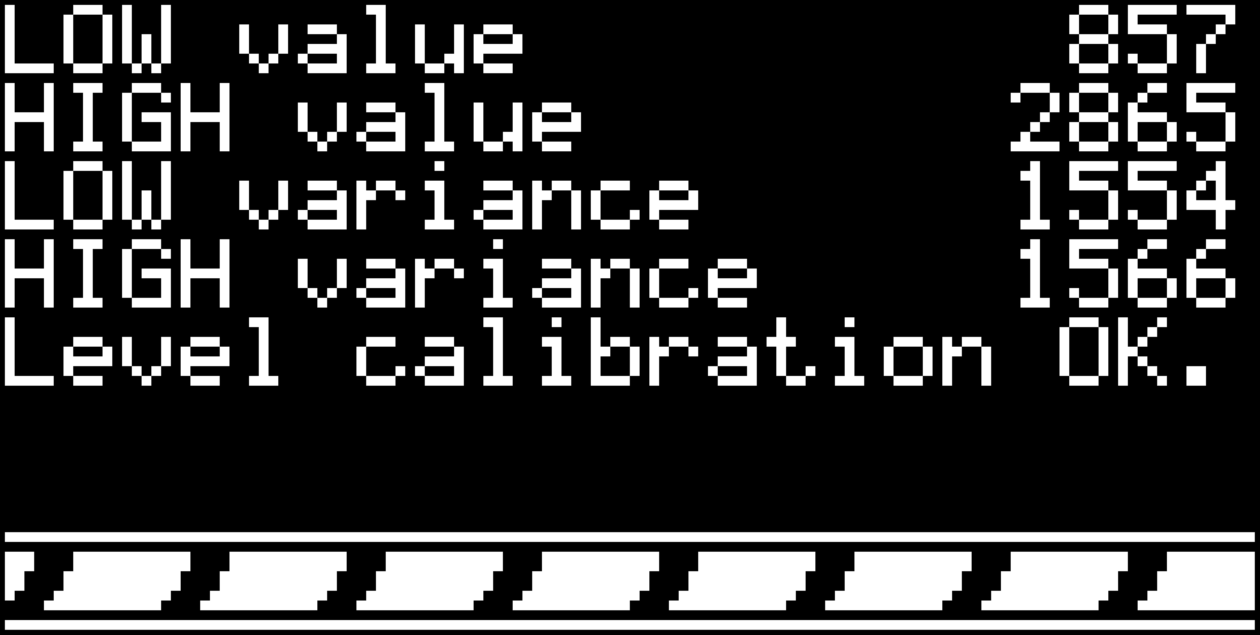
GUI on the device itself


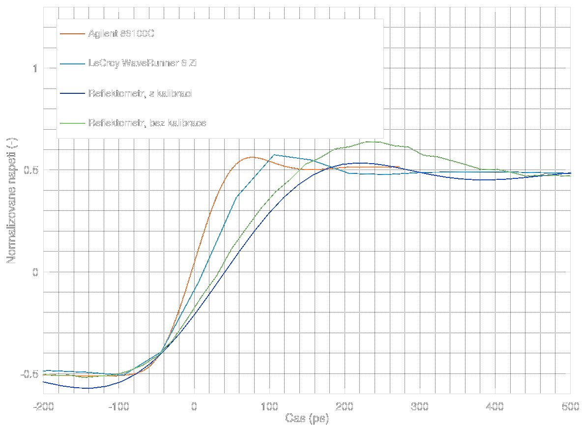

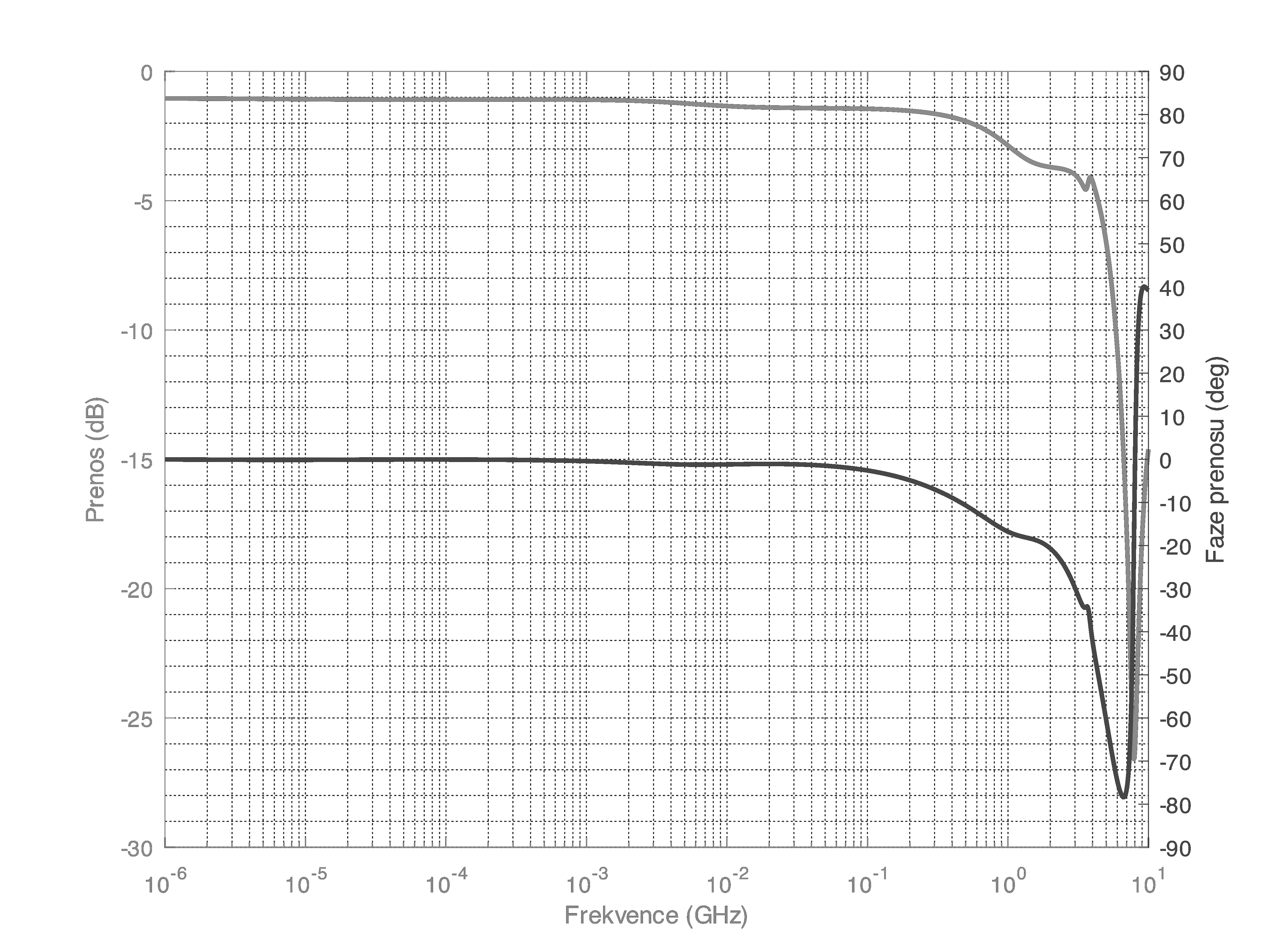
 Test port impedance
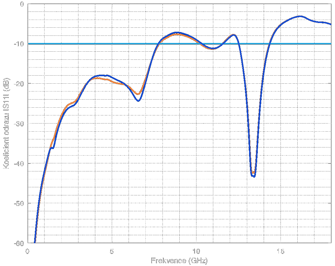
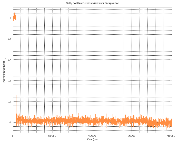
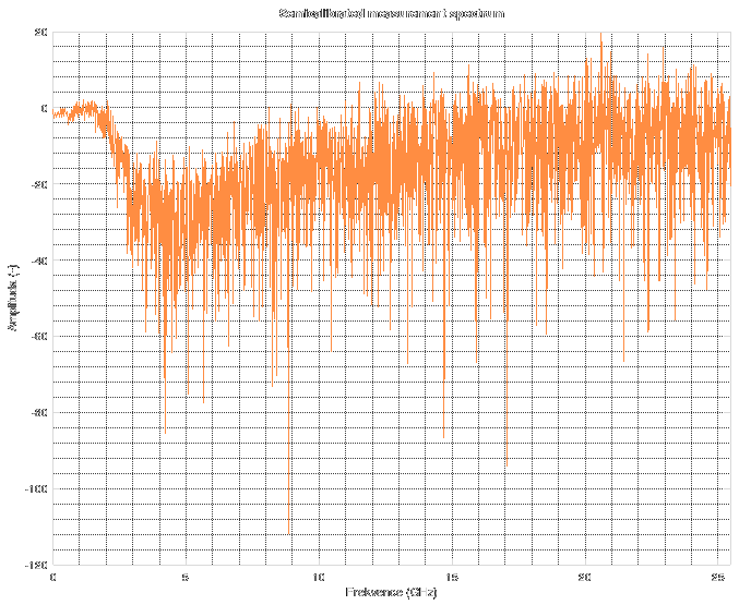
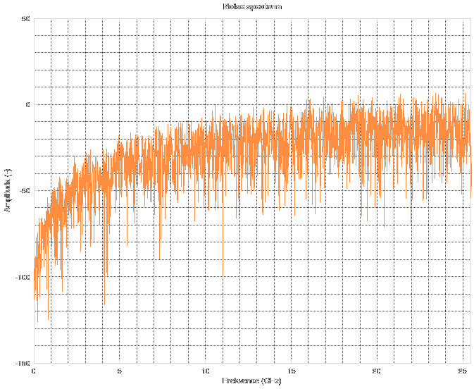
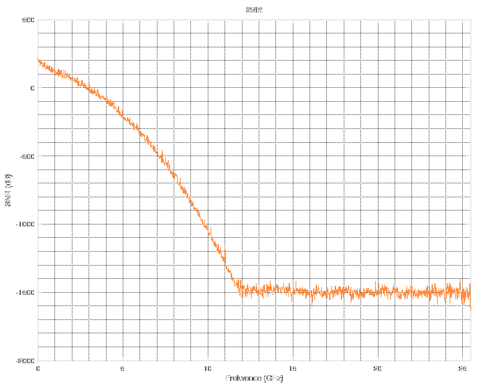
 Forget about the spectrum above 11 GHz. The noise floor corresponds to "near-zero" values in floating-point computations during FFT. Simply said, it is the noise floor of floating point numbers. When you do something in floating point, stay aware of the fact that its precision is not infinite. There are cases when you might run into this issue and then you have to resort to arbitrary-precision mathematics which can be slow as hell.
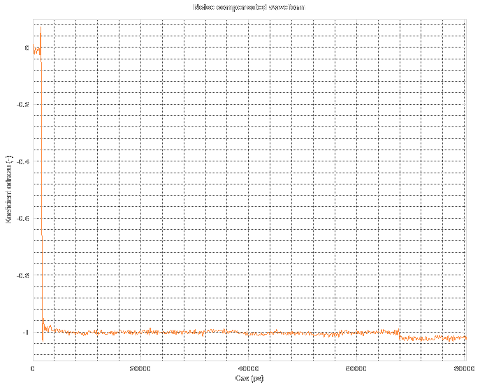
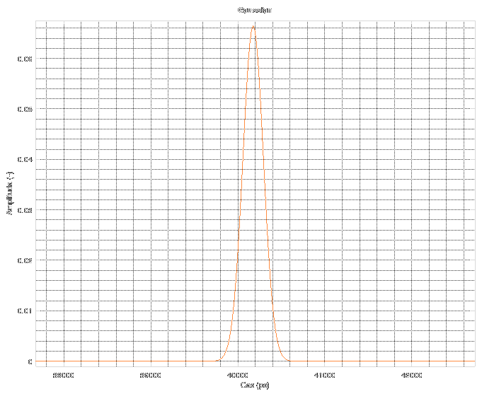
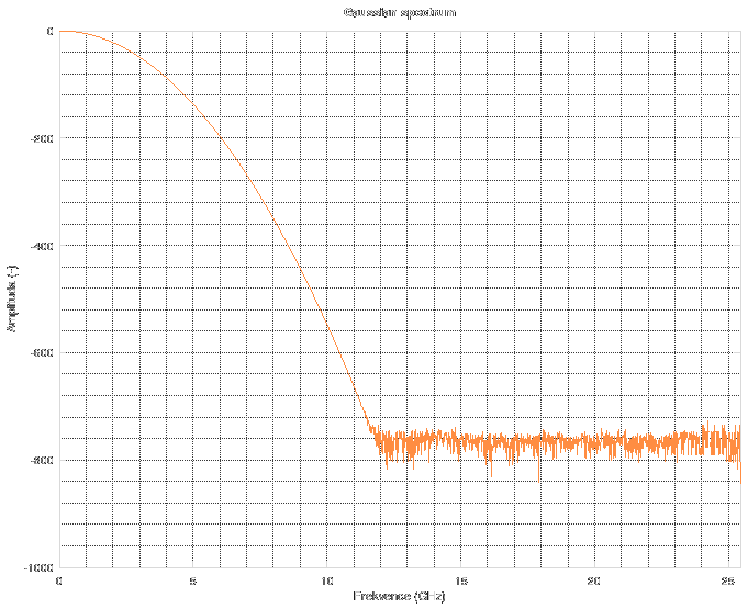
 The resulting Wiener filter looks the like this.
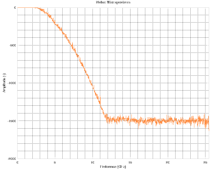
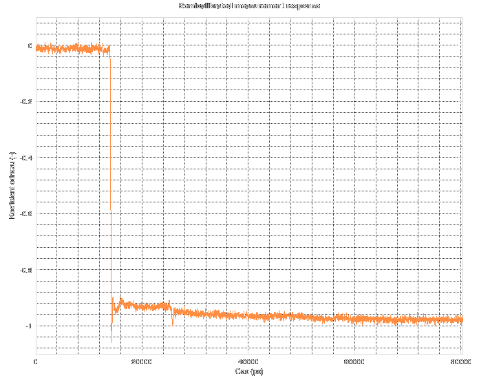


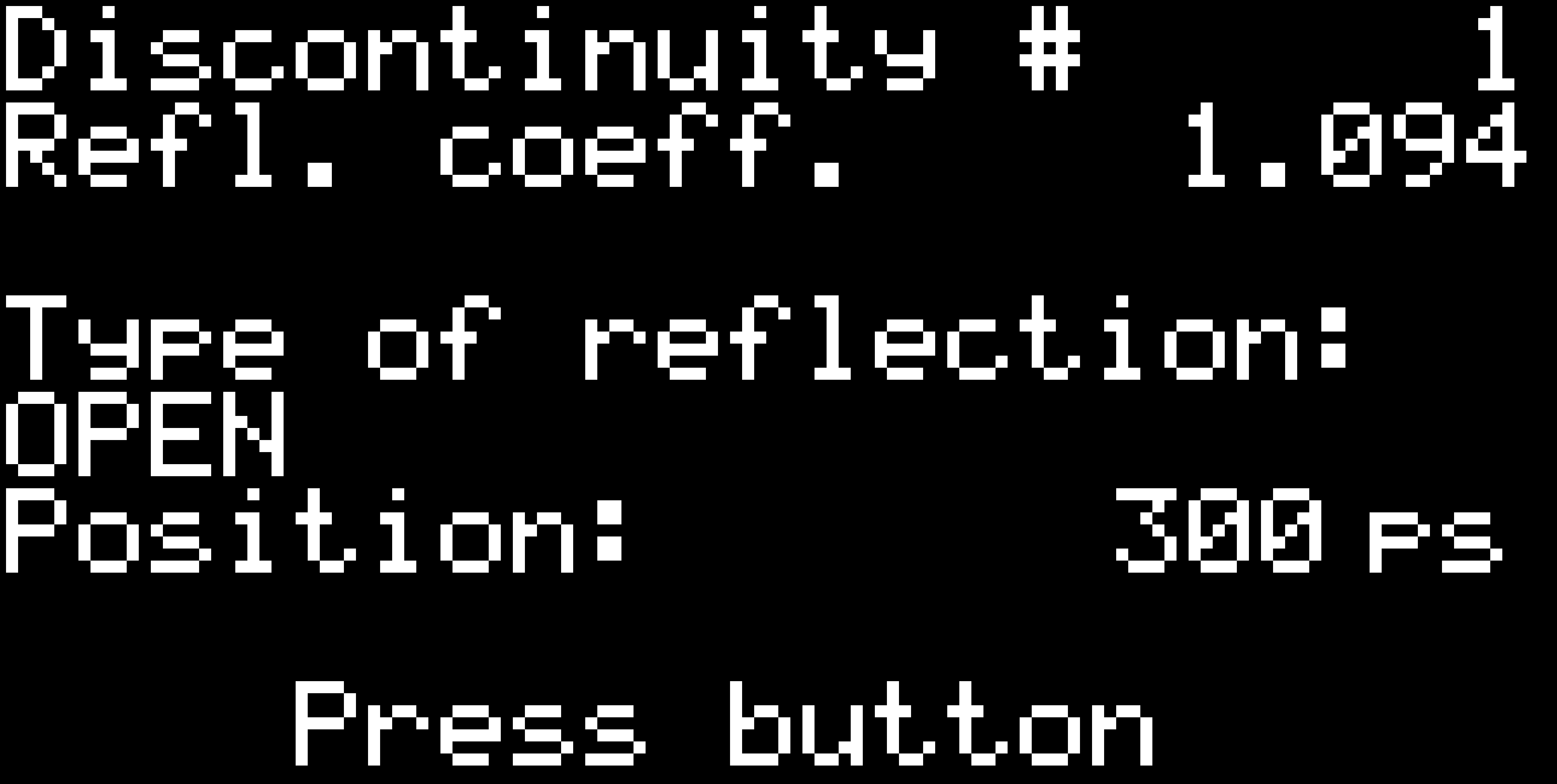 As you can see, it tries to detect the type of the discontinuity. It can detect "open", "short", "doubled impedance", "halved impedance" and for other cases it only shows "higher impedance" or "lower impedance".
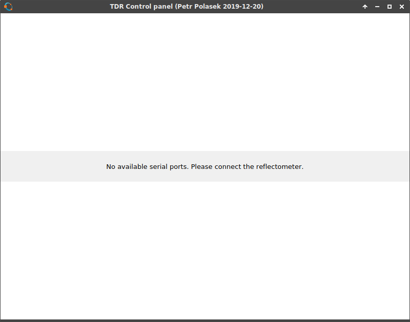 And it can even tell you if you are running the Octave binary from Flatpak with restricted access to serial ports and tells you how to correct it.
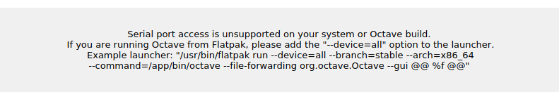
 After a handshake is performed, the GUI tells you the version of the firmware (time of compilation) and then finally connects to the reflectometer.

 Hugh Brown (Saint Aardvark the Carpeted)
 Simon Merrett
 Bruce Land
 Ben Hencke