Intro

As you might have already noticed, the hardware is quite simple. Usually this either means you are looking at a non-complete prototype which will need additional bugfixes or that there is a lot of work done by software. This project aims to be of the second kind, however I won't pretend it shows some signs of the first kind.

Synchronous sampling on STM32F103

"An image is worth a thousand head-sratches." It's quite obvious how to use external ADC triggering on STM32F1 from the image. Or maybe not at all. Let's start by stating that you have to enable the ADC, connect it to appropriate input pins, connecting the trigger to EXTI11 and configuring the NVIC to handle ADC interrupts. More after the image. You might want to make yourself a large mug of coffee.

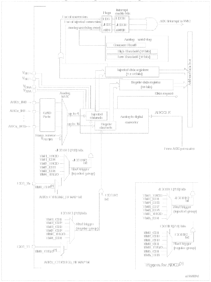
First you have to enable the clock to the port with analog pins and AFIO (alternate function configuration peripheral). Then set the analog pins as "analog inputs" and the trigger pin as "floating input" or better connect a pull-up or pull-down. For those familiar with STM32 - if you were expecting the trigger pin to be set as "alternate function", you were wrong. It doesn't work that way. In any case, don't expect to find this piece of information in datasheet or reference manual. Then you have to remap the trigger of ADCs to the external trigger on EXTI11 input. Maybe it will seem simpler once you see the source code (there is no code to enable clock to the ports used, because they are already on).

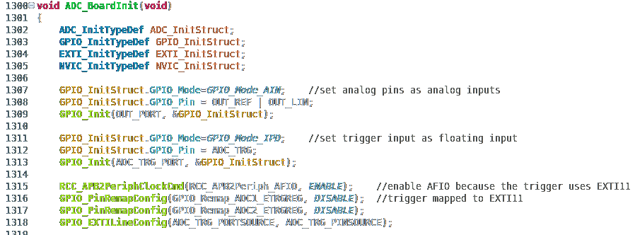
At this moment, it is all connected together, but can't trigger yet nor measure anything. What's missing? The trigger has to be enabled and the trigger condition has to be selected. ADC must be enabled, configured and calibrated. Interrupts need to be configured and enabled.

So just set up the EXTI to react to falling edge on EXTI11 and initialize it. Enable ADC clock and set the ADC to trigger using the external trigger. Then set the sample time length and initialize the ADC. Then it has to be calibrated (internal procedure of the microcontroller). Then one has to wait for the calibration to wait. An anti-optimization measure is included. Then enable the ADC interrupt, configure NVIC to watch the ADC EOC interrupt flag and enable it.

Now the microcontroller is ready to measure voltage using the ADC after being triggered using the external trigger, then run an interrupt which does some magic with the result. It could also perform a transfer using the DMA, but there are reasons why I used just an interrupt.

Logic in the interrupt

I won't explain the whole logic in the interrupt, because the state machine is a bit complicated. Let's concentrate on the practical part of the job.

The measured data are 10 microseconds long and contain 500000 values 20 ps apart. Since the Si5351 PLL VCOs start with unknown phase offset, it is not known where the beginning of the measurement lies in the dataset. There is also one thing worth mentioning. One sample occupies two bytes and the whole dataset occupies 1 MB of RAM. The F103 has only 20 kB of RAM and you cannot allocate all of it for the sampled data. Therefore you cannot sample the whole dataset and then try to find something in it. It has to be done vice versa.

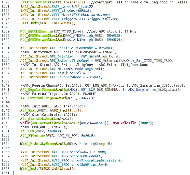
The interrupt tries to find a point where the data contains the largest derivation. Because of large amount of noise, it uses average of 16 first-order differences. After a bit of thought, an equivalent of this average is a difference of two values 16 points apart. The equation below should prove that.

Measurement plane position calibration

Now we will leave the interrupt for a while. During autocalibration phase, the firmware tries to roughly find the beginning of the dataset by collecting the position of the largest differentiation over several runs. Again, this is because of noise in the dataset. Then it asks the user to connect a cable. Then it performs several runs of measurement. In the measured data, the firmware tries to find the rising edge corresponding to the end of the cable. Using the voltage before and after the rising edge and its risetime, it selects a point before the rising edge as starting point of the measurement.

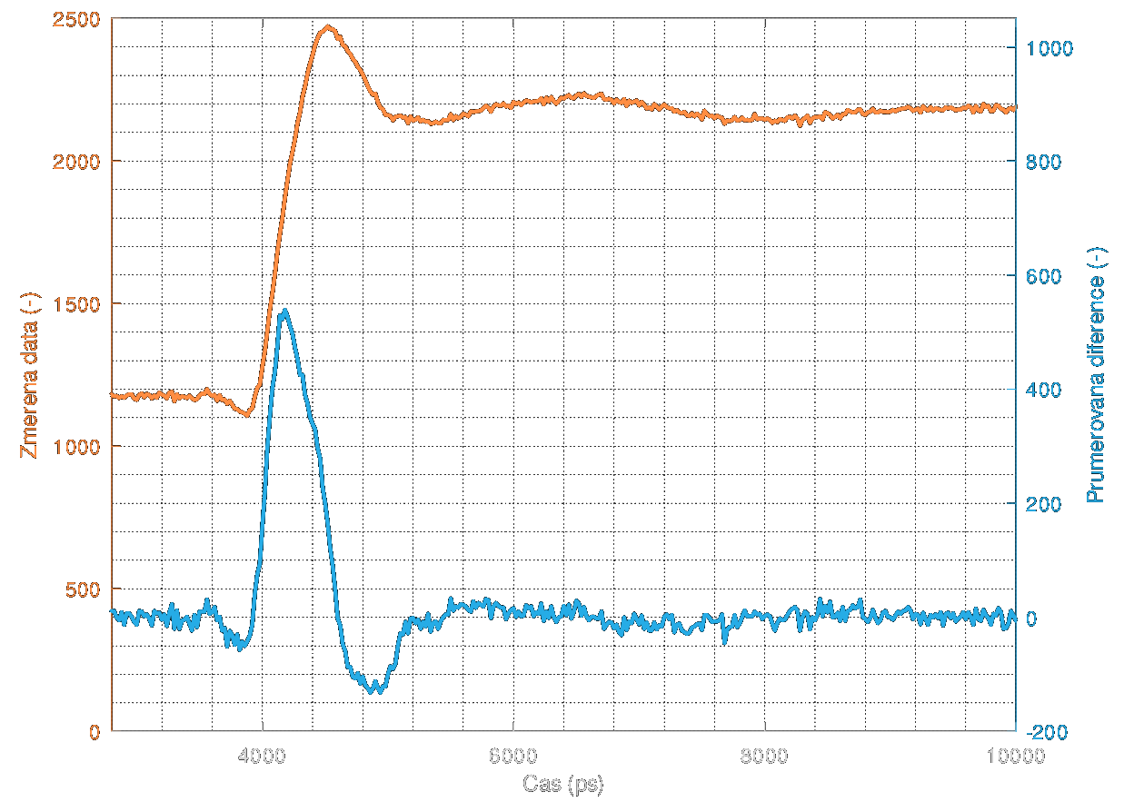
Back to the interrupt. To see what the interrupt sees from the differentiation, look at the next graph. The peak in the middle of the rising edge is quite easy to detect. The measured data are orange while the difference is blue. Again, sorry for Czech captions.

DC offset autocalibration

Before this part of autocalibration, there is one thing to do. The buffer amplifier with BF998 has its current source driven by DAC. The firmware first increases the current until the voltage during HIGH logic value gets safely under the higher limit of the ADC range. Then it measures the voltage during the LOW logic value. The current is increased/decreased until both voltages are symmetrically far from the half of the range of the ADC.

Noise level estimation

During the DC autocalibration, 4096 measurements are performed for each logical value. This gets a quite precise average voltage. Then, another 4096 measurements are performed which are used to calculate variation of the measured data. This serves as noise level estimation.

Averaging

The firmware uses averaging method which was used in 1980s in oscilloscopes made by HP. It stores only the averaged dataset and not all of the runs performed. If you are thinking it's "moving average", it's not. That would require storing all the measured runs. Exponential moving average would be closer. However the algorithm changes the weight of the stored data and new measurement so that in the end, the result is an arithmetic average of all the runs. And some noise caused by rounding errors.

The algorithm can be seen in the next equation. i is the current number of runs, x is the current sample and y is the stored data.

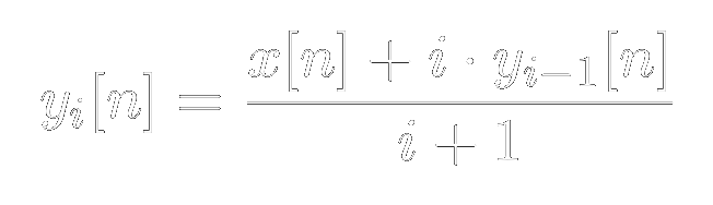
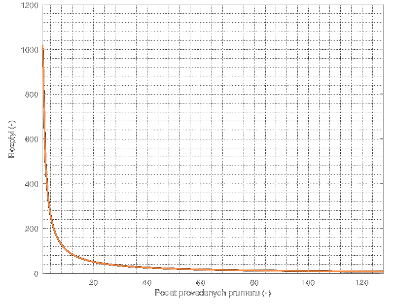
You might be curious what the averaging does to variation. The variation decreases as a function 1/N where N is the number of averages performed.

This function looks the same both when run in floating point and when run in integer mode. Not so when you look closely. If you multiply the variation by number of averages, you should get a constant function. Well, that happens when you run the averaging in floating point. When run with integers, you can expect some dark magic to start happening. And it does. The blue line is a differentiation of the variation while the orange line is the variation multiplied by the number of averages.

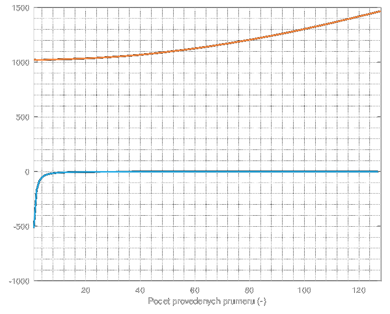
Oh boy, that's bad. You probably expect a lot of noise to emerge when running more than 50 averages or so. And yet you are completely wrong. The increasing curve only means that the noise gets dominated by the rounding errors instead of the measurement noise. Therefore, the noise present in the dataset is getting lower and lower until it hits a lower limit imposed by the rounding error. The noise could be theoretically as low as a few LSB. So, no big trouble. However, there is an optimal amount of averaging. You can see that the noise doesn't get much lower after more than 10 averages. And the rounding errors start to rise after more than 20 averages. These numbers change with the variation on the beginning. Or more precisely, on its square root - that's the standard deviation you are familiar with.

The optimal seems to be between around one half of the standard deviation.

Level autocalibration

During the DC autocalibration, the values for LOW and HIGH logic levels on the pulse generator are measured. These voltages should be equal to voltage measured after OPEN and SHORT calibration standards. And it works... quite enough. You can see the response to open end of cable.

It's not perfect, but good enough for automatic finding of discontinuities.

Discontinuity detection

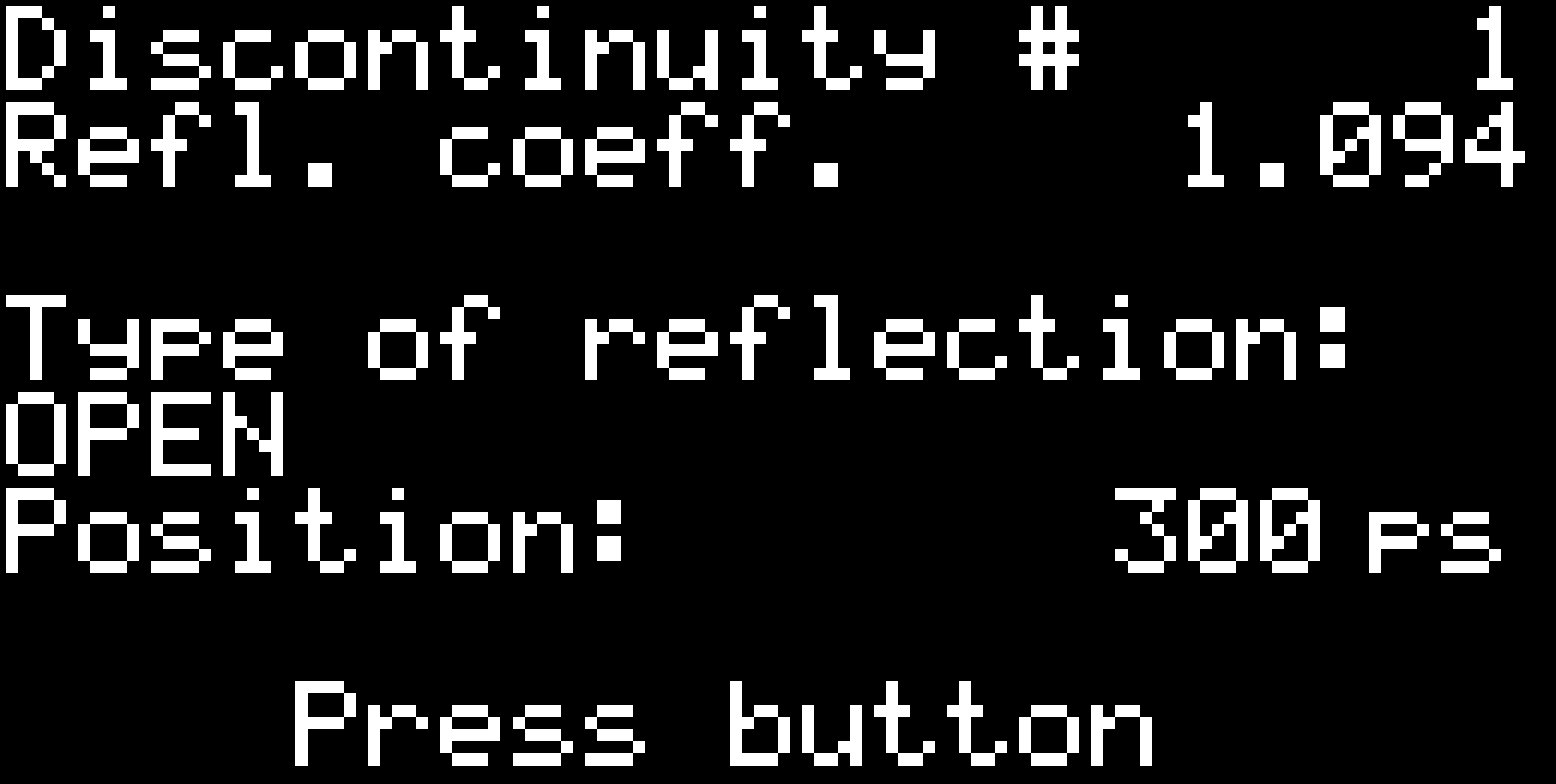
The software measures the dataset, then tries to find the largest differentiation point. Then it tries to find the next largest differentiation point excluding some tolerance field around the first discontinuity. This happens 8 times. The differentiations get sorted by the time they appear on (yes, I used bubblesort, no need to implement anything faster here). It's not very precise due to the limited calibration, but good enough to detect simple discontinuities. On a properly calibrated reflectometer, reflection coefficient outside the range <-1;1> should scare you. But since this is not properly calibrated, it's kinda OK.

See you next time. The next post should concentrate on the user interface on both the device itself and the Octave application.