 MS-BOSS
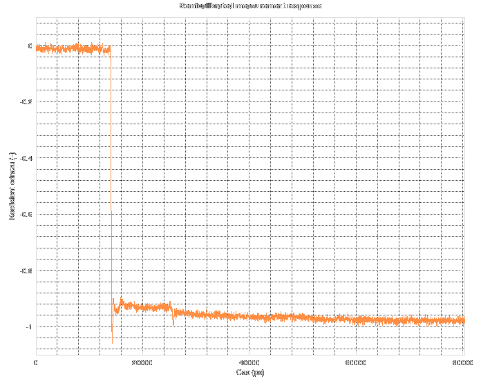
When I was talking about the Wiener deconvolution last time, I had it implemented, but not properly covered by analysis and graphs and therefore it did not contain as much information as I would like. A part of this appendix will repeat some statements from the last log, but in more detail and better-looking graphs. So, let's start with a graph of the measured spectrum. This one is a "semicalibrated" spectrum, which means that the "load" calibration has already been subtracted from the measurement, however the proper SOL calibration was not performed. The amplitude is logarithmic (and therefore in dB).
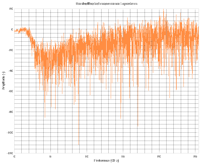
As you can see, it is not normalized to 0 anywhere in the spectrum. The spectrum looks kinda flat until 2 GHz, then falls off rapidly. Between 3 and 4 GHz, the signal completely sinks into something really nasty. It looks like random noise. Because it is. The reflectometer has useable frequency range up to about 2 GHz, then its response falls off and the rest of the spectrum is just random garbage not related to the measurement.
So you might ask how the noise spectrum really looks like. Here it is.
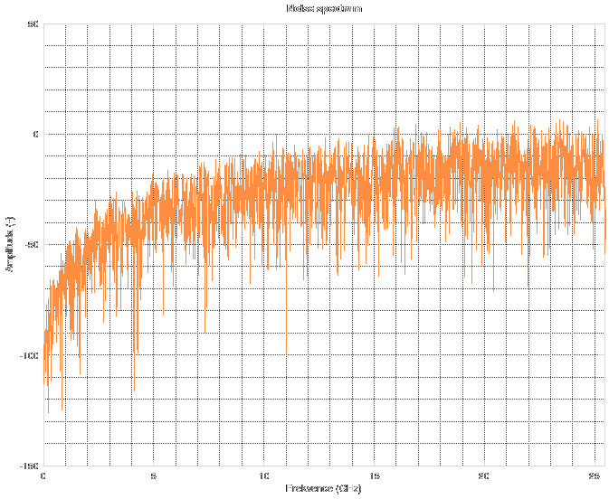
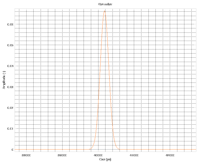
At low frequencies, it is quite subtle, but rises fast until about the 5 GHz mark, then stays almost constant. This is used for the estimation of SNR. The second part needed for SNR estimation is a Gaussian pulse or more specifically the probability density function which is a quit good model of derivation of the rectangular TDR impulse. Its best property is that once you integrate the pulse, you obtain a single real number, which is exactly 1. That means that you don't have to bother yourself with proper scaling of its spectrum amplitude-wise. Its spectrum starts at 0 dB and then falls off. The shape of the pulse is on next graph. Its width was figured out by experimentation asa compromise between amount of noise and effects of restrained spectrum on the data (pre-echo on edges, smoothed out features, longer risetime etc.).
And its corresponding spectrum looks like this. Again, it is logarithmic and in dB.
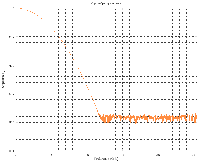 Forget about the spectrum above 11 GHz. The noise floor corresponds to "near-zero" values in floating-point computations during FFT. Simply said, it is the noise floor of floating point numbers. When you do something in floating point, stay aware of the fact that its precision is not infinite. There are cases when you might run into this issue and then you have to resort to arbitrary-precision mathematics which can be slow as hell.
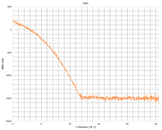
The gaussian spectrum and noise spectrum can be divided (element-wise, not matrix-wise) by each other to obtain SNR. You can see the estimated SNR in next graph, Y axis is logarithmic again. See how it reaches 0 at about 2.5-3 GHz. This is the point from which nonsense data prevail.
 The resulting Wiener filter looks the like this.
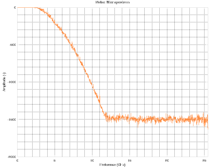
As you can see, its response is unit (Y axis is logarithmic) and then it sharply falls off above 2 GHz. This means that anything above this frequency is cut off. The cutoff frequency and the shape of the filter depends on the estimation of the TDR pulse.
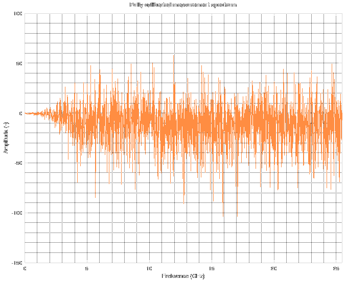
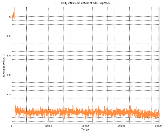
After the SOL calibration, the spectrum of the measurement looks like this. From about 1.5 Ghz you can see a fast onset of noise.
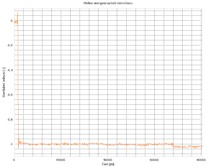
So, what happens if the Wiener filter is applied? The resulting spectrum is on the next graph.
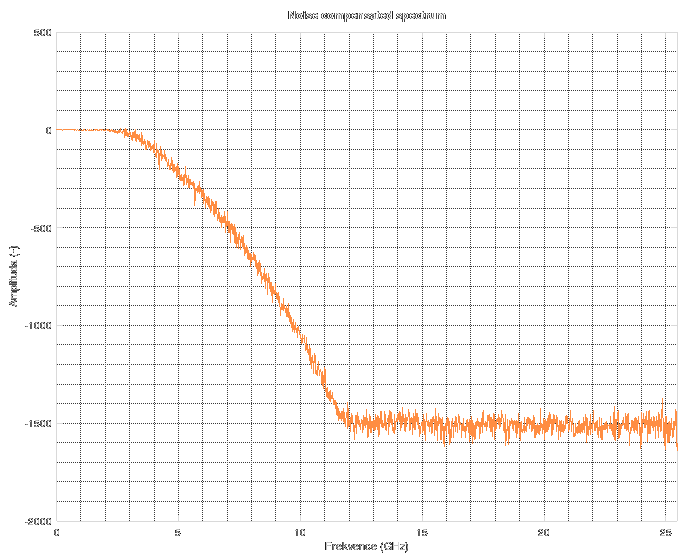
As you can see, the calibration is "somewhat valid" up to 2 GHz and then it gets cut off by the Wiener filter. What does it do to the measured data? The measured data are on the next graph.
Nasty, isn't it? The large falling edge is response to short on the end of cable. As you can see, it does not reach -1. Then, you can see another, smaller reflection about 12 ns after the first one. That's a reflection caused by the reflectometer's test port having wrong impedance (about 35 Ohms for the footprint of the SMA connector). Then it somehow slowly creeps to the -1 mark. Sadly, I do not know the origin of this effect. Dielectric soaking? Maybe, but not expected on high-quality cable. Heating of the driving transistor inside the CML buffer? Could be.
Then, it gets corrected by the SOL calibration and the noise gets amplified. The reference plane position also gets corrected. It is non-zero after the calibration, because the short is connected after another piece of cable which delays the reflection. However, the peaking and resonance after the falling edge is gone. The secondary reflection caused by the reflectometer's non-ideal impedance is gone (which is THE ONE reason why I implemented the calibration). The slow "creeping" movement of the response is gone. Noise appears and also a new artifact on the end of the waveform - this is where the original data ends and the rest is only an approximation of future.
And when the filter gets applied...
As you can see, all of the out-of-band noise was removed and now the data starts to make some sense. You can even distinguish easily the point at 68 ns where the original data used to end. Now, the response is quite properly placed and scaled on both the 0 and -1 marks. The peaks on the falling edge are mostly due to effects of the restricted spectrum. The peak BEFORE the edge is completely made up by the calibration and noise reduction techniques, as it was not present in the original uncalibrated data. The peak AFTER the edge could partially be caused by the numeric operations, but it was substantially reduced compared to the original data.
You might be curious how the noise reduction affects the measured rising edge of the reflectometer. Let's have a look at a graph which will be also mentioned next time when I show some more measurements performed on the reflectometer.
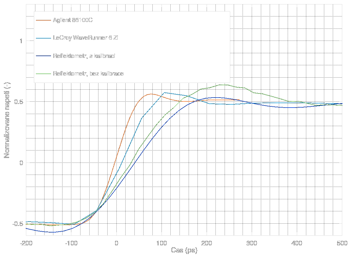
The fastest rising edge belongs to the Agilent 86100C with TDR/sampling plug-in installed. It shows the real rising edge as emitted by the CML buffer. This is the reference for all the other traces.
The next slower one belongs to LeCroy Waverunner 6 Zi oscilloscope. The rising edge is quite fast, but slower than on the Agilent. However, even though LeCroy boasts its capability to sample "up to 40 GSa/s", it does not. Its samplerate is about 25 GSa/s and we were really trying to get the highest possible sample rate. Nope, not going to happen
The next, slower one is the reflectometer without calibration and noise reduction. You can see slower risetime, larger peak after the edge and some noise.
The last one is the reflectometer with calibration and noise reduction. Noise is gone, overshoot damped, everything is smoothed out. Risetime is slightly slower and preshoot appears. However, nothing dramatic.
Next time, I will probably have the master's degree exam done (planned for 6.2.2020), so I will probably finally write about the measured parameters (most of them were already at least once mentioned in logs) and about the result of the exam.
If you are sensitive, please do not read further. If you are thinking about buying any product of LeCroy, read further but be warned that several words from fecal vocabulary can be found throughout the text (I am not English-native so I could come up with maybe 30 words of this category in my language, but not in English, sorry).
<RANT ALERT>
Honestly, the Lecroy is a piece of liquid sh*t which feels like it just came out of someone's a*se and still has a bit of. I wish I had a fast oscilloscope, but honestly, I would rather have a pile of t*rds sitting on my table than this piece of cr*p. It has one omnipotent semi-rotary-joystick-button-piece-of-rotten-sh*t as the main control.
And it is sooo ridiculous even though I owned 2 oscilloscopes, have everyday access to another 4 scopes in our makerspace, many others in my work and each made by different brand, so I should probably know how to use oscilloscope. Nah, that doesn't happen with LeCroy. It's even worse than the Agilent oscilloscope which lets you save a screenshot but delays the saving by several seconds which leaves you time to open some menus and then it saves the screenshots with the menus overlayed...
I can control right about any of the microwave measuring devices at the school department. Vector and scalar analyzers? Check. Noise analyzers? Check. TDRs and TDTs? Check. Various generators, detectors and any other possible equipment? Check. LeCroy t*rd? Not at all.
Trust me, I have used sh*tty chinese oscilloscopes with wonky rotary knobs which sometimes skip steps or do random magic due to noisy edges. These are bad, but still OK. Really, when something which costs nearly the same as the house you live in, you expect it could be more useable than chinese cr*p which costs about $500. Once you try to fiddle with any settings, you find out there is NO BUTTON TO GET BACK TO CHANNEL SETTINGS. Really. I tried pressing any and all of the buttons. I COULD get back to the channel settings, but either via some non-deterministic way of pressing buttons as if I was playing Mortal Kombat or Tekken. Sometimes, I could get back by disabling that channel and enabling it again. Sometimes not.
And the rest of the interface is as bad as this single piece of it. Look, if you want to know how a good minimalist interface looks, get your hands on the HP54100 from 1989 (!). Everything is deterministic and always has the same place. Everything, even the measurements, fits on the CRT and does not have to be placed in the graph area where you either cannot read it or it masks the trace. It was made in 1989, is driven by a Motorola 68000, has a CRT, less RAM than you ESP8266 and even then it is substantially than the Lecroy. Stay away from any blo*dy piece of en*ma which has a sticker "LeCroy" on it.
</RANT ALERT>
Discussions
Become a Hackaday.io Member
Create an account to leave a comment. Already have an account? Log In.