 Timothy Kanarsky
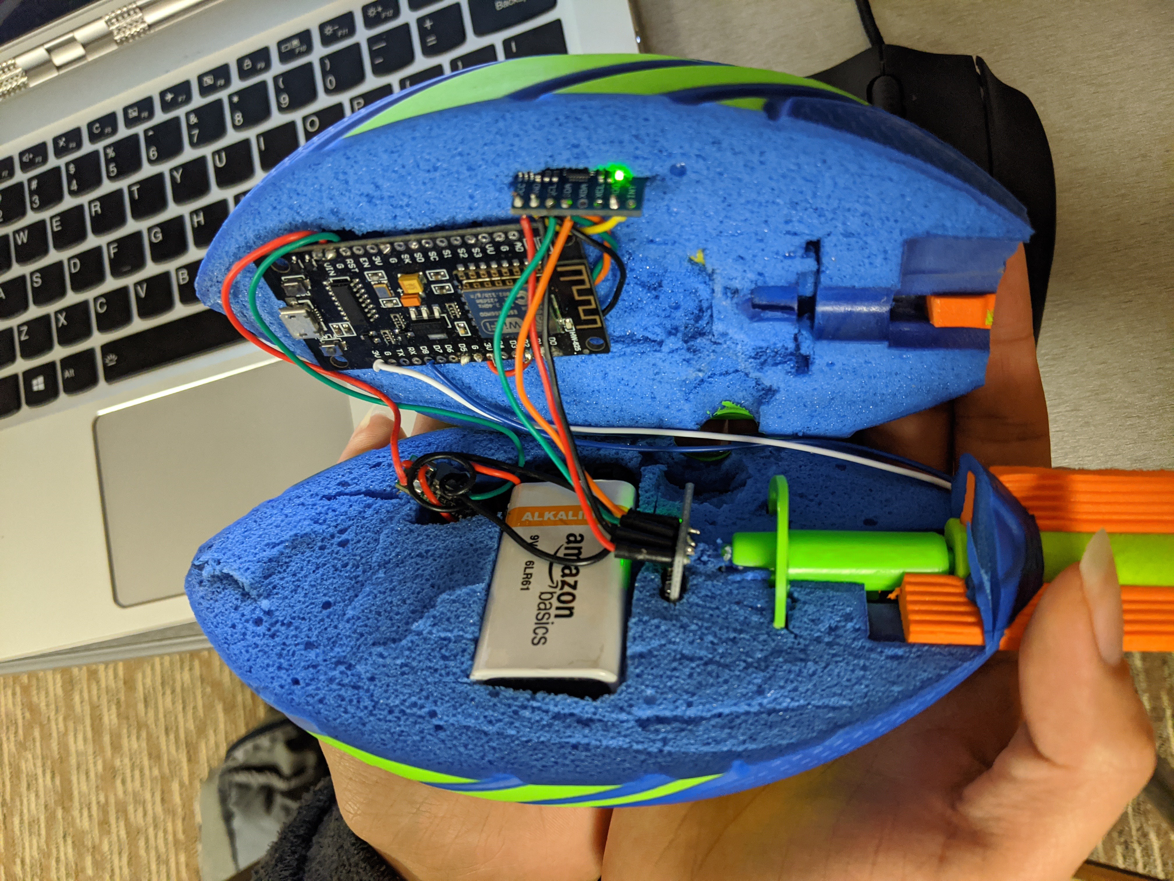
We started the project by slicing the body of a Nerf Vortex foam football in half with a box-cutter. We chose this particular football because it was cheap, stable during flight (due to the dart-shaped tail) and easy to mount electronics in. The ball had three whistles mounted along its perimeter; we removed one to make room for the electronics.
We had two goals: measure the acceleration of the ball during the throw (which is used to calculated distance thrown) and measure the centripetal acceleration of a point on the ball (which is used to calculate angular velocity).
We needed to use two accelerometers, as it's impossible to distinguish linear acceleration from centripetal acceleration given a single acceleration vector.
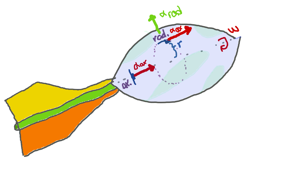
We mounted one of the accelerometers along the axis of rotation, taking great care to place the accelerometer chip as close as possible to the spin axis. This was our axial accelerometer, which would be unaffected by centripetal acceleration during flight (at least in theory).
We began by calculating the initial velocity of the football. This was done by integrating the magnitude of the football’s axial acceleration during the throw (from start time to time of release) and subtracting the acceleration due to gravity.
Next, using the angle at which we threw the football (with respect to the horizontal) we calculated the horizontal component of the ball's velocity:
and integrated it once more, from time of release to time of catch.
This double-integration is a direct application of the fundamental theorem of calculus to bring us from the realm of accelerations (measured in meters per second per second) to the realm of distances (measured in meters). The accuracy of this method is severely limited in the long run, as any errors in the accelerometer readouts tend to be magnified over time and result in greater and greater drift in the absence of absolute positioning data. However, this dead-reckoning method can be decently accurate -- most ICBM's rely on precise accelerometers and gyroscopes to calculate their location and bomb the right targets!
The other accelerometer was mounted two centimeters away from the spin axis in the widest part of the ball, normal to its surface. This was our radial accelerometer, which would experience a great deal of centripetal acceleration during flight.
We took the magnitude of the radial accelerometer's data, which eliminated the effects of position on the acceleration readout. This calculation is done on data points collected in mid-air, where the centripetal acceleration is the only significant component of the radial acceleration vector (no gravitational acceleration, negligible tangential acceleration, negligible linear acceleration)
Using the angular acceleration and radius of rotation (the radial accelerometer spins in a four-centimeter-wide circle) we calculated the linear velocity of how fast the ball spun:
Finally, we divided the linear velocity by the radius to determine the angular velocity of the football.

The setup runs on a NodeMCU with an ESP8266 processor. We chose this microcontroller because of its low profile (no through-hole components or headers) and built-in WiFi modem.
- The NodeMCU has a 3.3 volt logic level, unlike the Arduino Uno’s 5 volts. Fortunately, all our components ran fine on a reduced voltage, though the beeper was quieter.
Two MPU6050 digital accelerometers were attached to the I2C bus on the NodeMCU.
- The accelerometers have a default address of 0x68, which would’ve caused an address conflict, so we shorted the AD0 pin to 3.3V on one of the accelerometers to switch its address to 0x69.
- These accelerometers are configured, by default, to a range of +/- 2 g (~20m/s^2) of acceleration per axis, but are capable of measuring +/- 16 g (~160 m/s^2) of acceleration. As our project would deal with abrupt changes in velocity, we switched the accelerometers to the latter range.
A piezo beeper was attached to a digital output on the NodeMCU to signal logging start/stop.
A button was attached to a digital output on the MCU to trigger logging start/stop.
A 9-volt battery powers the MCU through a switching regulator to convert the 9 volts from the battery to a steady 3.3 volts.
The electronics are press-fit into notches cut into the foam body of the football. To power the circuit on and off, we simply connected and disconnected the battery.
We originally planned to add an indicator LED and toggle switch to quickly turn the unit on and off, but never got around to it.
The NodeMCU pulls acceleration data every ~5ms from the two accelerometers, which it maps to calibrated m/s^2 values and stores in memory. It also creates a Wi-Fi hotspot and serves its clients (our computers and phones) a static web page containing the collected data and a few scrolling graphs.

When the button is pressed, the ball goes into logging mode. Comma-separated data points (consisting of calibrated x, y, z acceleration data for both radial and axial accelerometer and a timestamp) are continuously logged to onboard storage until the button is pressed again. The NodeMCU runs an FTP server that allows us to pull these .csv files into our computers over the same Wi-Fi connection we used for monitoring, allowing us to log faster.
The default partitioning scheme on the microcontroller allocates two megabytes of flash storage for logging. We had to clear the filesystem every few throws (once again, over FTP) to keep it from filling up.
As this was a physics class, not a digital electronics class, we had to test our creation in a controlled experiment. We measured out 4, 8, 12, 16, and 20-meter intervals, and took turns the ball back and forth. Every few throws, we pulled csv files from the microcontroller and wiped the filesystem.
The csv files were imported into a numpy array, and the acceleration magnitudes for both accelerometers were plotted on the same axes. We went through the datasets and manually tagged the start of throw, end of throw, and catch timestamps. We calculated the delta-times between each timestamp, with end-of-throw/catch delta serving as the time of flight and the start-of-throw/end-of-throw delta serving being used later on in the integration. To calculate the initial velocity, we integrated the axial acceleration using the numpy.trapz() function (a Riemann sum discrete approximation of the integral below the curve). To calculate the average angular velocity, we averaged the angular velocity data (calculated using the above formulas) over the time of flight. We repeated this step for each trial for each distance.
The resulting data looked something like this:

Both acceleration values spike during the windup and throw, and the magnitude of radial acceleration was significantly higher than the magnitude of axial acceleration.