 EK
EK
To predict how our robot may perform in the real environment, a physics model would be useful to understand the forces at play. The calculated results serve as data points that can be verified experimentally to see how they differ in the real world.
---> EJA v2 Physics Model on Google Sheets <---
Highlights
Here's the key points from the calculations:
- In order for the weight to buoyancy ratio to be > 1.0, the mass of the entire robot has to be at least ~6 kg (13.2 lbs)
- Hydrostatic pressure at 30 m (100 ft) is 43.89 psi - roughly half of what we hypothesize as the limit for the Nalgene container
- At 50 m (164 ft), it is 73.16 psi, which would be an excellent test
- When the buoy reaches the surface, the tension on the line is 46.61 N, and the buoyancy-to-weight ratio is 1.25
- Based on the robot's total mass of 6.0 kg, with an initial velocity of 0 m/s:
- Terminal velocity is ~0.76 m/s, or 2.7 km/h (1.7 mph)
- Landing force is ~-8.5 N, or almost 2 lbf
- To reach 5 m, it takes 6.5 seconds
- To reach 30 m, it takes 39.1 seconds
- If freefalling for 1 min, the robot would descend 46 m
- To reach 1000 m, it would take 21.7 minutes
- (At that point, the pressure at 1000 m is 1468.95 psi though!)
To improve the physics model calculations, we will verify experimentally:
- Mass
- Buoy
- Rope spool
- Entire robot
- Ballasts
- Percentage of buoy submerged when at the surface
- Descent time
There are scenarios of what we want to calculate:
- Buoyancy
- Terminal velocity
- Drag force
- Freefall velocity - Descent time to target depth
- Hydrostatic pressure
- Tension of the rope
Let's dive in to each scenario!
1. Buoyancy
The weight to buoyancy ratio is the key number to making sure the robot will sink.

Buoyancy is all about the volume of liquid displaced by the robot. This is why a steel boat can still float, yet a steel ball will sink - because of the volume. The density of the material does not matter.
The volume of the robot is estimated to be 4753 cm^3.

The minimum mass must be 6.0 kg to get the weight-to-buoyancy ratio to be > 1 (meaning, it will sink). For a mass of 6.0 kg, the weight-to-buoyancy ratio is 1.169.
The addition of ballasts was added in CAD to fine tune the position of the centre of mass. Further experimentation will need to be completed to ensure that it is the correct amount of ballasts to achieve 6.0 kg.
In CAD, we see the estimation of the mass to be 12 kg. However, skeptical of that number based on the real world materials. Actual mass will need to be confirmed experimentally when the robot is entirely constructed.
Thanks to Leo for the post from last year that breaks down the buoyancy topic very well!
2. Terminal velocity
A large terminal velocity could impact the robot by inducing vibrations when landing, having a risk of unseating the magnet wiper. As well, imprinting the seafloor. Minimizing this would reduce those impacts.

Based on a mass of 6.0 kg and a target depth of 5 m,
The terminal velocity for the robot is 0.766 m/s. For comparison, that is ~70% of the typical human walking speed (2.5 mph).
Although there is no term for depth, the model does change as the density of water changes when going deeper. For seawater, the linear change in density was extrapolated from this table (Source: Encyclopedia Britannica). The scale of the change is very small: 0.01 m/s total difference from 0 m to 10,000 m depth.

The drag coefficient was selected to be 1.55. This is based on the inverted triangle shape, which the robot somewhat looks like given the diameter of the handles on the upper stage are larger than the diameter of the lower stage. (Source: Sighard Hoerner, Fluid Dynamic Drag via Wikipedia)
Another way of minimizing terminal velocity would be to streamline the design, thereby reducing the coefficient of drag and area.
3. Drag force

As the robot is descending through the water, there is a drag force pointing upwards against the robot.

What we expect to see is drag and weight balance out at some point. Sometimes this can happen before the target depth is reached. For this model, there is a drop-off around 5 m. This graph shows the difference between the drag force and weight. This approaches 0 as the forces balance out.
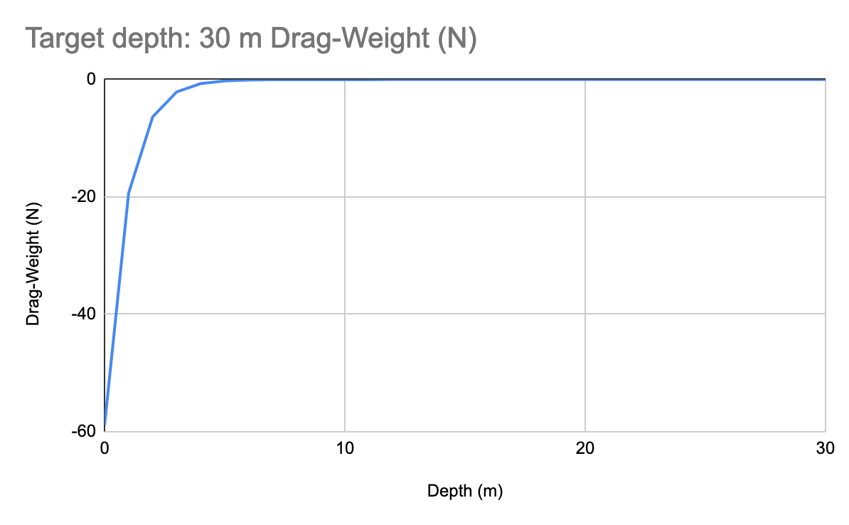
The freefall velocity is a term in the drag force equation that plays a role in this. This will be discussed in the next section.
Something that is concerning is a different scenario where the robot is entered in to the water at a 90 degree angle. Meaning, it's not pointed down, it's on its "side". The drag force will be different as the area will change along with the coefficient of drag.
Verifying experimentally the behaviour of the centre of mass will be useful in determining if more work is necessary for such edge cases. User feedback will be useful in seeing how often those edge cases happen in reality (perhaps they happen more often than not!).
4. Freefall velocity - Descent time to target depth
How much time the robot takes to reach the target depth depends on the freefall velocity. Freefall velocity is also a term that is used in the drag force formula.

Note: In the physics model, the square root is taken on the above formula to obtain the v value.
Assuming the robot starts with an initial velocity of 0 m/s,
To reach a depth of 30 m it will take 39.1 seconds. For shallow water testing of 5 m, it will take 6.5 seconds. To reach 1000 m, it would take 21.7 minutes. Wow!

The relationship appears linear for the most part because the depth where freefall velocity approaches terminal velocity is 2.88 m.
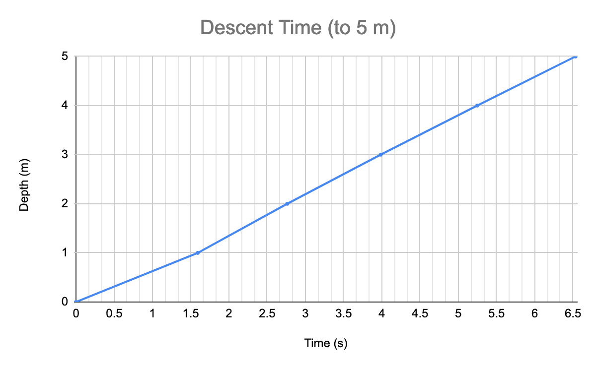
The non-linear relation is evident in the first 5 m (you have to look carefully around the 1.5 to 3 second mark, but in the numbers it is evident).

This is controlled by the exponential decay term in the formula for drag. In that, y represents the current depth. In our model, we used a ratio of current depth to target depth as y.
The formula for freefall velocity where the independent variable is distance is derived from freefall velocity as a function of time. The full derivation can be found on Hyperphysics here.
As mentioned in the previous section, the drag force balances out with the weight force after a portion of time, and that is controlled by the exponential decay term.
5. Hydrostatic pressure
Hydrostatic pressure increases with the depth. This is of importance since if the pressure is too much for the material, the buoy's Nalgene enclosure will be destructively compressed or shattered.

Our hypothesis is the current buoy enclosure might withstand ~80 psi (based on this video). This would set 50 m as the depth limit at 73.16 psi with the buoy in its current configuration. In the upcoming shallow water testing, it's predicted the pressure would be ~7 psi.
Depth (m) | Hydrostatic Pressure (psi) |
5 | 7.31 |
30 | 43.89 |
50 | 73.16 |
100 | 146.35 |
1000 | 1468.95 |
10000 | 15238.97 |
Going from 50 m - 500 m, and onwards, a different enclosure strategy for the buoy will be needed.
6. Tension of the rope
The rope is the vertical line that goes from the base on the seafloor to the buoy on the surface. If this rope is under a lot of tension, this also cuts into the whale when entangled and swimming. This is why some ropes have weak links or weak insertions, which break after a certain amount of force, so the whale won't be dragging the gear along with it.
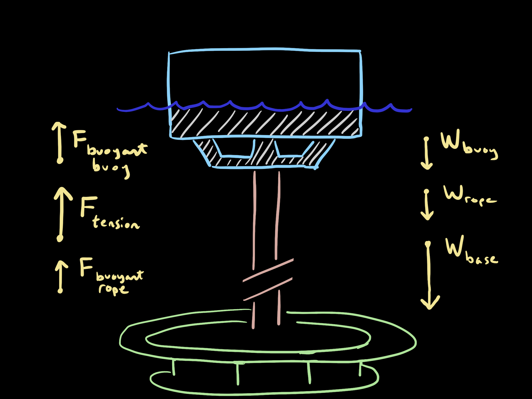
The tension force points upwards, countering the weight of the buoy and rope. It is assumed that the buoy is submerged 50% when it is at the surface — which influences the volume calculation for buoyancy. The mass of the buoy and the mass of the rope is assumed to be 0.5 kg each (this is a wild estimate, and needs to be verified in reality).

Based on the robot mass of 6.0 kg, an entire spool of 30 m, and the buoy submerged by 50%:
The tension on the rope is 46.61 N, or 10.47 lbf.
That is approximately 1/16th the tension on a piano string.

While looking at these numbers, it would also be beneficial to see the buoyancy-to-weight ratio to ensure the buoy will float. The buoyancy-to-weight ratio is 1.25, meaning the buoy will float with this rope.

There are a lot of variables at play here where the model probably falls short. For example, fishers may use weighted line, and the diameter may be larger. There may be water currents that pull the buoy away from the base. Verifying experimentally will allow us to see the validity of these calculations.
Assumptions and errors
Some assumptions in this physics model are:
- Assumption about drag force only balancing out when reaching the target depth
- Using a ratio of depth/target depth in the exponential decay term for freefall velocity
- Miscalculations in volume (for example, if excluded bodies in the model were included when Fusion 360 calculates this — further investigation is necessary)
- Cross-sectional area for drag force (would this be an average of the lower stage and upper stage area? or the largest area?)
- Coefficient of drag was set at 1.55 based on a cone that is larger at the top (source)
- Extrapolated a linear formula of density of seawater for the various depths (source)
- Assuming the drag force balances out at the target depth, this would mean that the landing force would always be the net force
- Skeptical of the mass estimation in Fusion 360
As a flaw, this physics model addresses the "best case" scenario. Namely, when the robot is oriented in the proper direction and enters the water from rest. A next step could be to try to model what happens when the robot enters at a 90 degree angle, and when the robot is submerged with an initial velocity. Observations through trial and error in real world testing can help with adapting the model for those scenarios.
Conclusion & Next Steps
It has been an absolute blast to prepare this model, reviewing these concepts again. This gives some data points to compare the real world testing to. Eager to test to see how far off the results actually are.
Next steps are to test this in the real world and see how it performs, and adjust the model as necessary.
Any mistakes in here are my fault. Know something that could be better? Leave a comment below :)
Discussions
Become a Hackaday.io Member
Create an account to leave a comment. Already have an account? Log In.