First I had to choose some parameters that would determine the specifics of the scimitar antenna. The 4 that I chose were a horizontal scaling coefficient, inner and outer curve values and scale. The code to create the scimitar geometry looked like this:

def scimitar (scale,a1,a2,a,segment,h):
  A = np.zeros((2*segment,2))
  for i in range(0,segment):
    t = np.pi/(segment-1)*i
    x=scale*np.exp(a1*t)*np.cos(t)
    y=scale*np.exp(a1*t)*np.sin(t)
    A.itemset((i,0),a*(x-scale))
    A.itemset((i,1),y)
  A.itemset((segment-1,1),A[segment-1,1]+h)
  for i in range(1,segment):
    t = np.pi/(segment-1)*(segment-i)
    x=scale*np.exp(a2*t)*np.cos(t)
    y=scale*np.exp(a2*t)*np.sin(t)
    A.itemset((i+segment-1,0),a*(x-scale))
    A.itemset((i+segment-1,1),y)
  A.itemset((segment,1),A[segment,1]+h)
  A.itemset((2*segment-1,0),0)
  A.itemset((2*segment-1,1),0)
  return A

where scale, a1, a2, and a were to be optimized though the evolutionary algorithm and segment and h were to be held constant at 15 and .001 respectively. I set boundary conditions for the antenna so that they would be a reasonable size (Not good ones though because the output antenna ended up being about a meter long). Next, I modified the existing code to test the scimitar geometry and output its score as a sum of all of the VSWRs in the chosen range to optimize. Essentially, you would be minimizing the average over a range. After running it for 500 generations with a population of 500 the end result looked like this:

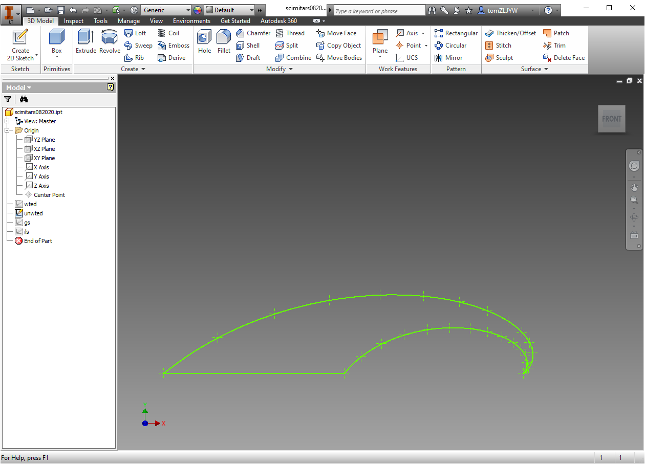
which gave a VSWR graph that looked like this:

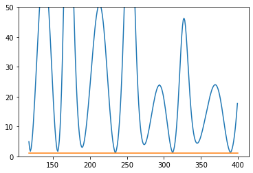
where the y-axis is 0-50 and the x-axis is 118 to 400MHz. After that I tried a few other optimization strategies. First, putting a 3 times weight on all frequencies higher than 250MHz which yielded this antenna:

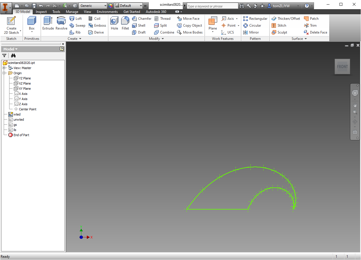
and gave a VSWR graph of:

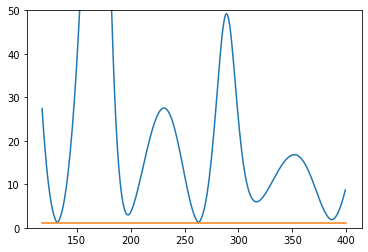
(same axis). Next I wanted to see if real versions of the antenna would give similar VSWR plots as the simulated ones. After drawing out the scimitar shapes on some paper, gluing tinfoil to that paper and cutting out the shapes, I tested the geometries. Side note: tinfoil gives the same VSWR values as a metal plate of the same shape, antennas are just made out of .032" aluminum so they don't melt. Outlines of wire also (supposedly). give the same VSWR as a filled in sheet. Anyways, the VSWR sweeps of the physical antennas were completely different from the simulated ones. The actual sweep of the weighted looked like this:

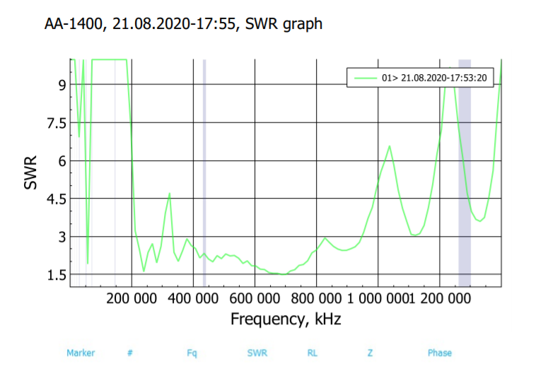
the x-axis is 0-1400MHz the shape is sorta similar in the range 118-400 but the values are considerably lower in the real world. This is sorta ok because if the shape of the graph is similar then an optimized version will still be optimized in the real world and just have a better VSWR.