 pjkim00
I've been interested in control systems for a long time. The convergence of math, electromechanics, sensors, and programming holds a place dear to my heart. Last year, I built this low budget ball balancing platform with my kids. The ball position is sensed using a resistive touch screen picked up for $1.50 at AllElectronics. The platform is tilted using micro-sized hobby servos, $2 each. Add an Arduino for a few bucks, a steel ball, wires and a battery holder and the total bill of materials was under $20 and came together in an afternoon.
It initially started off using PID (proportional, integral, derivative) control using the Arduino and it worked reasonably well after finding the correct tuning parameters. I had ideas of converting to state space control-- using linear algebra to control stuff. It then sat on a shelf for a while until I saw an article on HaD titled, "Talking Head Teaches LaPlace Transform."
https://hackaday.com/2020/08/09/talking-head-teaches-laplace-transform/
Steve Brunton has a bunch of videos on Youtube including a series called "Control Bootcamp." There are plenty of videos about control theory but precious few showing actual implentation. I wanted to see if I could actually get this to work.
How hard could it be?
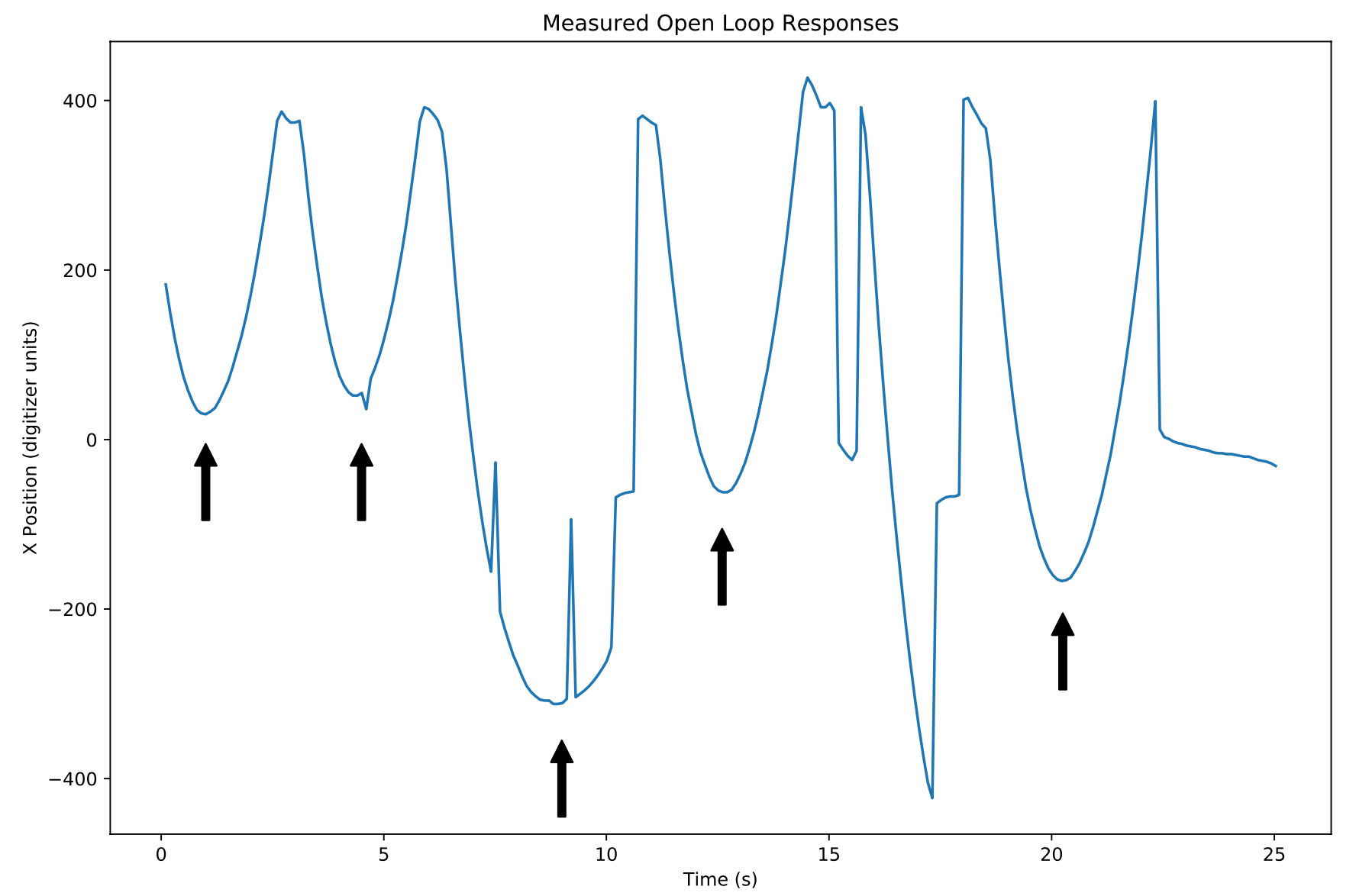
- Measure the dynamics of the ball balancing platform.
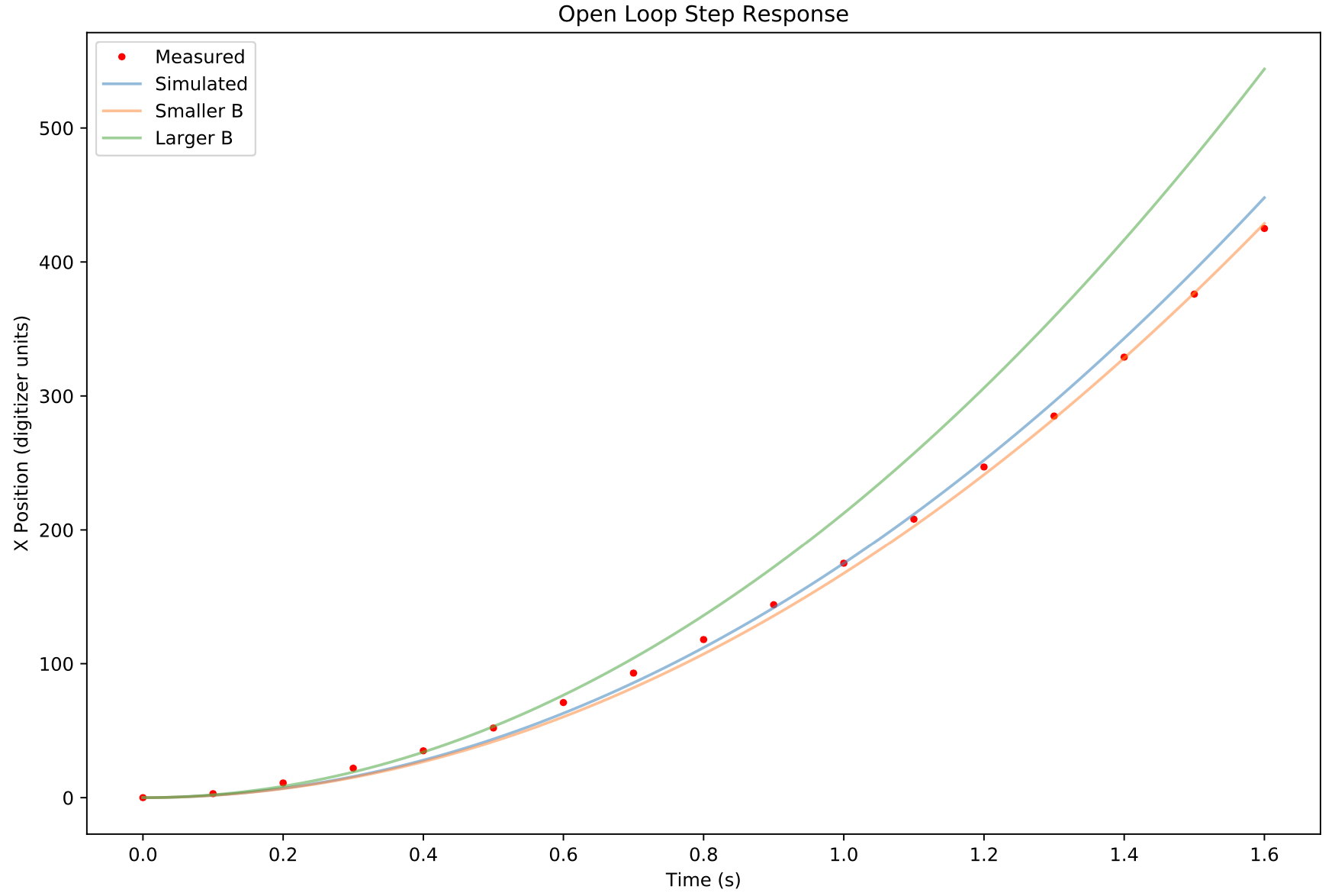
- Come up with a set of equations describing the dynamics of the system.
- Convert to state space matrix form
- Convert continuous time system to discrete time system
- Simulate using the python control library to confirm correct dynamics
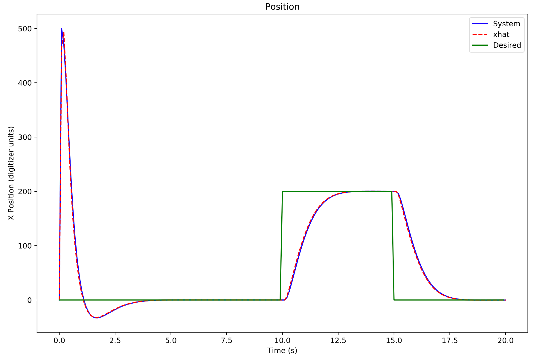
- Design an observer
- Design a feedback system
- Simulate some more to confirm it works as expected
- Convert above simulation to Arduino
- Tune parameters
- Tune the model
- Iterate above a lot
- Profit!
I found the entire process in turns daunting and not so bad. I would like to share some of the things I learned along the way. The python control library (https://python-control.readthedocs.io/en/0.8.3/) was very helpful. It provided almost all of the functionality of Matlab for this kind of work.
I think I bit off a little too much the first time around. I tried to use a Kalman filter as an observer because the resistive touchscreen sometimes glitches (perhaps from small dead spots in the resistive layer). I also tried to use a linear quadratic regulator for the full linear quadratic gaussian (LQG) enchilada. I want to go back to these at some point.
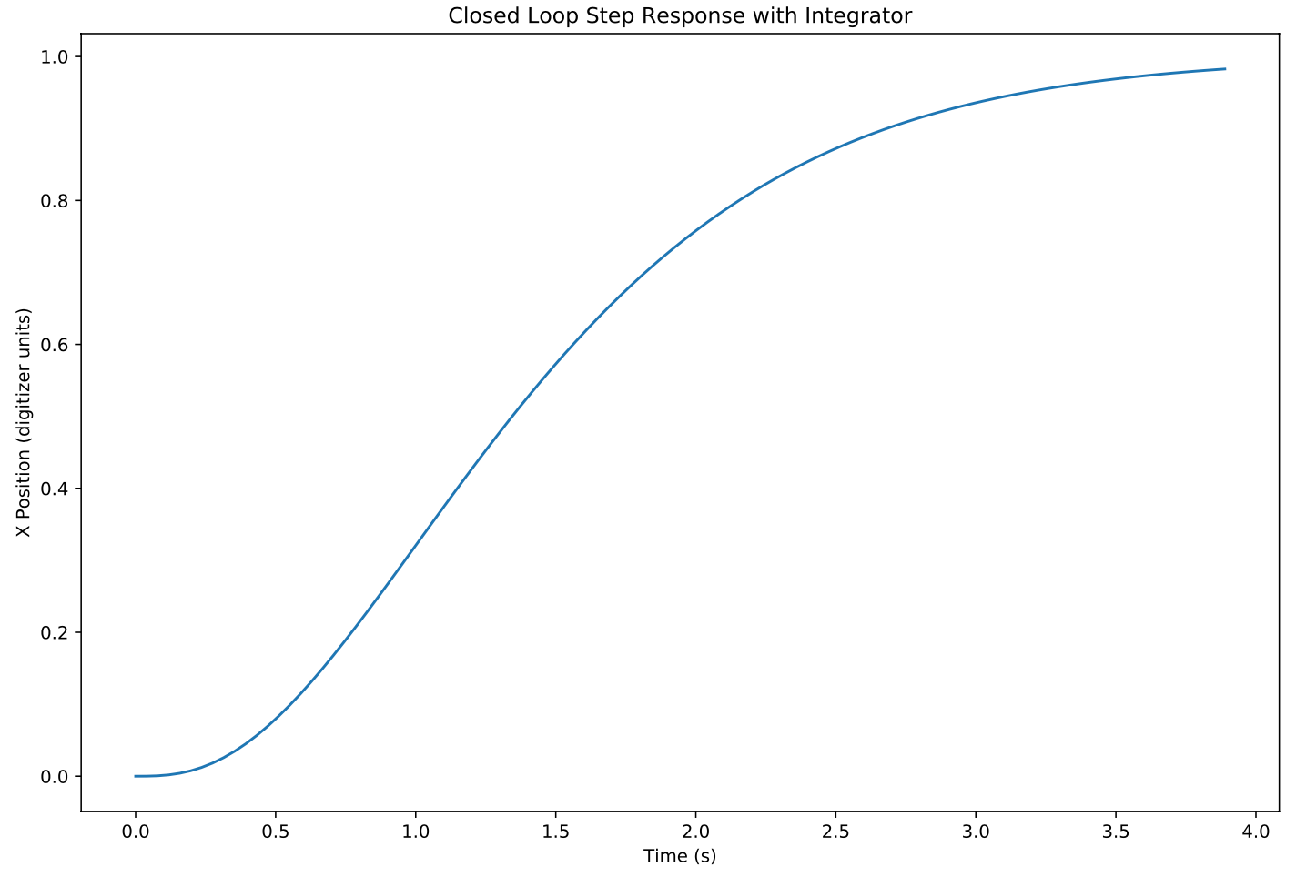
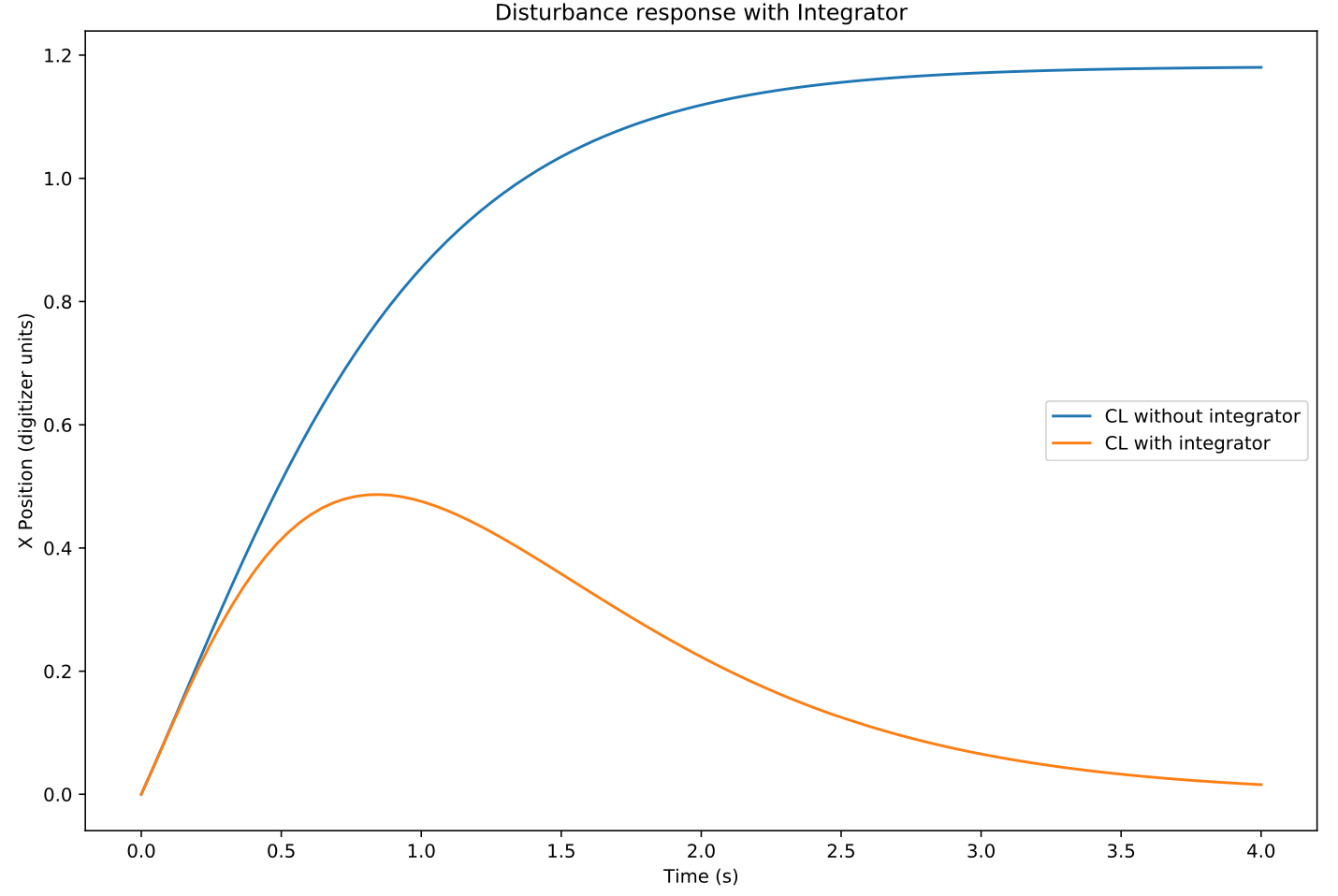
I had tantalizing hints of success. After a lot of parameter tuning and more trial and error than I care to admit, it worked-- sort of. I had naively believed that the magic of state space would take care of steady state errors. The steady state error of plain vanilla state space control is horrible-- i.e. any deviation from the ideal dynamics described in your equations will lead to steady state error. But the magic of state space control has solutions for this in the form of robustness methods.
You can see the platform in action here:

 Tim van Iersel
 James Harding
 hIOTron
 Bobby Christopher