 Phil Malone
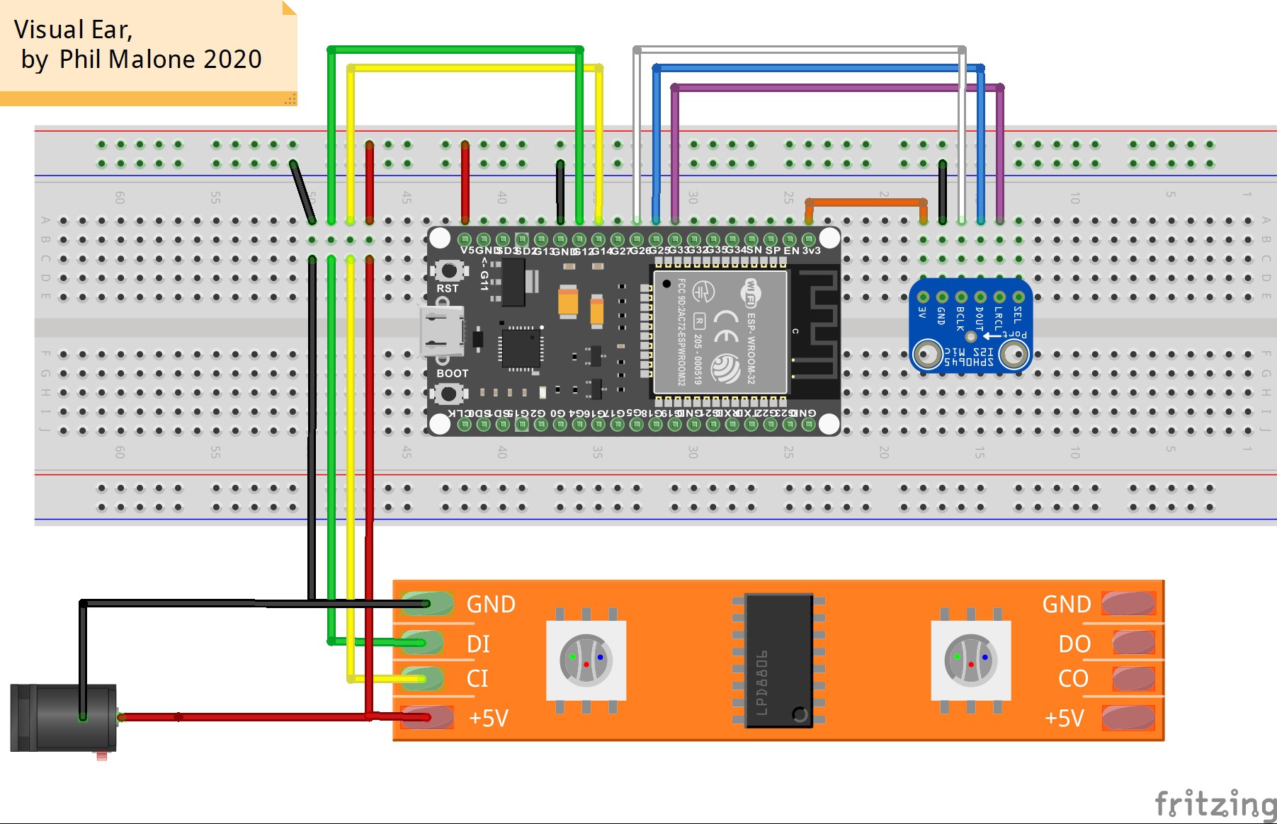
I’ve shown my basic setup in the Fritzing diagram above (this is a cool way to show my prototype setup). Note that I'm using the ESP32 Dev Kit with an I2S digital microphone and DotStar LED strip (which allows faster data clocking)
The problem:
Taken at face value, there is no way I can collect 4096 audio samples and then process them into 59 Bands and still get a reasonable display/response rate, based on my initial test data.
To get 59 discrete Bands in my desired 50-17,000 Hz range, I need at least 2048 Frequency Bins, which means I need to give the FFT twice as many audio samples at about 36K Hz. To just collect 4096 samples at 36 kHz will take 114 mSec (4096/36000). Then to run the FFT on these values would appear to require another 148 mSec. This would imply a display cycle of 262 mSec, or JUST four updates a second.
Given that my goal was to be lower than 50 mSec, this is completely unacceptable. So I had to develop some strategies for reducing these times. This is what I came up with:
Split the audio sampling and the FFT between the two cores.
Remember that the ESP has two processing cores. I’ve never used this before, but I knew that both IDEs enable you to pin tasks to specific cores. So I decided on a strategy whereby one core would be collecting audio samples while the other core was processing the previous sample. I implemented a simple semaphore between the two cores that would let them bounce between two alternating audio buffers. This approach would let me update the display after each FFT cycle without having to wait for another full audio buffer to be collected.
Speed up the FFT using lookup tables and single precision floating point.
The first thing that I noticed was that the Arduino FFT library was calculating the required FFT windowing function for every cycle. This involved trigonometric functions which were sure to be slowing down the calculation. I modified the code to run this algorithm once, during setup, and stored the weights in an array for later recall.
Next I saw that the Arduino FFT library was using double precision floating point (double) for its calculations, so I ran some tests to see if switching to single precision (float) would speed things up without affecting the output. I was pleasantly surprised to see a very large speed increase with little impact on the display.
Incremental audio Updates.
At this point I had reduced the FFT processing time down to about 16 mSec (a 9 x improvement) but my audio sampling was still slowing down the overall process. Since I could not sample faster (as it created unusable frequency Bins) and I could not collect less samples (as it produced less frequency Bins) I had to get creative. My problem was that until I have new audio data there was no point running the quicker FFT again.
My final solution to this dilemma was to sample the audio data in smaller Bursts, and then assemble them into a “sliding buffer” from the last “N” bursts. This way I could feed new data to the FFT more frequently while still having the same large number of samples. Using 4 bursts of 1024 audio samples worked well, but 8 bursts of 512 samples was even better.
I suspect sweat spot for this process is where a single burst takes about the same to collect as the FFT takes to run, that way the FFT algorithm never waiting for new data, and the latest data is extremely fresh. I’ll save this for future tweaking.
You can find the current code implementation here:
Discussions
Become a Hackaday.io Member
Create an account to leave a comment. Already have an account? Log In.