Close
0%
0%

Getting Cozy with the Diffraction Limit

Do you hate the diffraction limit when you take an image of a scene? Me too! Here is a story of trying to do my best to correct it!

Public Chat
Similar projects worth following
150 views
0 followers
Follow along as I work on imaging at and past the diffraction limit! :)

Here is the challenge!

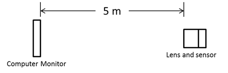
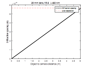
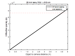
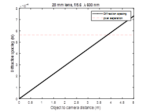
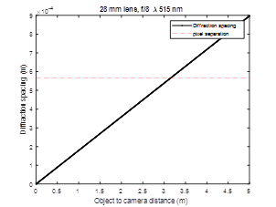
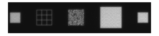
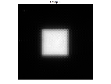
A computer monitor with a width of 0.475 m is placed at one end of room.  The maximum resolution of the monitor is 1680 pixels across the width, therefor the pixel width and height are approximately 283 um.  A lens and imaging sensor are placed 5 m away from the monitor, and the monitor is imaged.  The lens has a fixed focal length of 28 mm lens, manual focus ring, and manual f-stops at 2.8, 4, 5.6, 8, 11 and 16. The image sensor is a Sony IMX219PQH5-C.  This sensor was chosen because it has a relatively small unit cell size of 1.12 um.  The experimental setup is shown below.  I placed the results in the instructions sections.

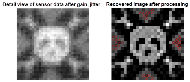
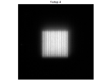
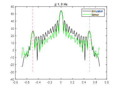
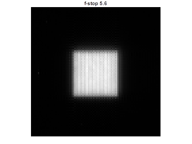
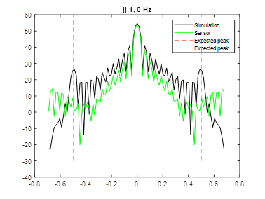
At the diffraction limit, I was able to reconstruct the image in the mean square error sense...yeah!

  • Mounting the raspberry pi (Sony) v2 sensor for use with a lens

    sciencedude199004/03/2021 at 15:29 0 comments

    You can 3D print a piece that can hold the lens and sensor.  Please see my other project:

    https://hackaday.io/project/177321-upgraded-lens-for-raspberry-pi-v2-camera

    Cheers!

  • Working with the raspberry pi v2 camera, raw and sliced data

    sciencedude199004/03/2021 at 15:28 0 comments

    The raspberry pi v2 camera (i.e., the Sony image sensor) is great since it has small unit size for the imaging pixels.  Getting the raw information from the sensor is straightforward, but speed is important for getting the training done on this setup.

    First thing - let's not burn the sd card!  So, if you are taking lots of images, create a ramdisk to place those images!

    First, make the directory:

    sudo mkdir /mnt/ramdisk

    Edit the rc.local file

    sudo nano /etc/rc.local

    Add the lines above exit 0

    mount -o size=30M -t tmpfs none /mnt/ramdisk

    /bin/chown pi:root /mnt/ramdisk

    /bin/chmod 777 /mnt/ramdisk

    Reboot, then check the file with

    df -h

    Now, start raspistill.  In this case, we will leave it running.  This way, you can take time lapse photos very quickly.  Here is the command (using MATLAB syntax, but you could start it with anything that can ssh into the pi):

    ['nohup raspistill -n -t 0 -drc off -ss ' num2str(shutter_time) ' -ex off -awb off -ag ' num2str(analog_gain) ' -dg ' num2str(digital_gain) ' -r -s -o /mnt/ramdisk/' f_name_img ' > /dev/null 2>&1 &']

    Next, get the process id from:

    pgrep raspistill

    And then to take a picture, you use a modified version of the kill command (strange, but it works):

    ['kill -USR1 ' num2str(raspistill_pid)]

    Next - as you might have noticed, I don't need the whole raw image.  I just need a part of it.  You can write a small python script that resides on the pi that can slice the raw image.  Once the .jpg file has been created, you run the python script to slice out what you need to produce a .bin file.

    ['python test.py -i /mnt/ramdisk/' f_name_img ' -o /mnt/ramdisk/' f_name_bin ' -s ' num2str(slice_row) ' -f ' num2str(N_slice)];  

    Here is the listing of test.py - pardon the indenting - you'll have to double check it if you use this script...

    #!/usr/bin/python

    # imports
    import sys, getopt, io, os

    # main, usage from the pi@raspberrypi command line:
    # python test.py -i /mnt/ramdisk/image_1.jpg -o /mnt/ramdisk/hi.bin
    def main(argv):
        inputfile = ''
        outputfile = ''
        startrow = 0
        stoprow = 0

        # Get the inputfile and outputfile, and the start and stop row from the input arguments
        try:
            opts, args = getopt.getopt(argv,"hi:o:s:f:",["ifile=","ofile=","snum=","fnum="])
        except getopt.GetoptError:
            print 'test.py -i <inputfile> -o <outputfile> -s <startrow> -f <stoprow>'
            sys.exit(2)

        for opt, arg in opts:
            print arg
            if opt == '-h':
                print 'test.py -i <inputfile> -o <outputfile> -s <startrow> -f <stoprow>'
                sys.exit()
            elif opt in ("-i", "--ifile"):
                inputfile = arg
            elif opt in ("-o", "--ofile"):
                outputfile = arg
            elif opt in ("-s", "--snum"):
                startrow = int(arg)
            elif opt in ("-f", "--fnum"):
                stoprow = int(arg)

        # echo the input and output file names
        print 'Input file is ', inputfile
        print 'Output file is ', outputfile
        print 'Starting row ', startrow
        print 'Stop row ', stoprow

        isfile = False

    # Better be a filename...
        if isinstance(inputfile, str) and os.path.exists(inputfile):
            isfile = True
        else:
            raise ValueError

        if isfile:
            # open the file and read the data, in bytes
            file = open(inputfile, 'rb')
            img = io.BytesIO(file.read())
       ...

    Read more »

View all 2 project logs

  • 1
    Diffraction

    Diffraction Limit

    The angle for the diffraction limit is:
    Angle = 1.22 lambda / D
    (source: http://hosting.astro.cornell.edu/academics/courses/astro201/diff_limit.htm) where  angle is the angle in radians, lambda is the wavelength, and D is the diameter. 


    Figure 2  Diffraction limit angle.
    The diameter, D, is taken to be f / f_num where f is the focal length 28 mm, and f_num is the f-stop setting for the lens (2.8, 4, 5.6, 8, 11, and 16).  For a computer monitor, the separation between two point sources can be as low as 2 times the pixel width, that is, approximately 565 um.
     

    Figure 3  Computer monitor point source spacing.
    If we consider a setup where we vary the distance between the monitor and the sensor, then we can find the diffraction limit for imaging the monitor.  For example, if the sensor was very close to the monitor, then the pixel spacing for the monitor could be very small.  The larger the separation between the monitor and the sensor, the larger the pixel size needed to be able to capture it.  The pixel spacing for the particular screen is shown as the horizontal dashed line.  The wavelengths were selected based on the peak responsivity of the imaging sensor pixels, 460 nm for blue, 515 nm for green, and 600 nm for red.  With a f-stop setting of 5.6, then we are very close to the diffraction limit at 5m.  Since the f-stop setting is mechanical, we can expect some error in the setting.  So, measurements will be presented for a setting of 5.6 and 8.


    Figure 4  Diffraction limit for a f-stop setting of 5.6.

    Figure 5  Diffraction limit for a f-stop setting of 8.
    Another way to understand the diffraction limit is by the considering the frequency response of the aperture.  This response is found to be something like sinx/x (source: https://scholar.harvard.edu/files/schwartz/files/lecture19-diffraction.pdf), which means that above a certain “frequency” of pixels (or spacing of two pixels), the information at the monitor will be cut off.  So, trying to go from the sensor data back to the image on the monitor will be ambiguous.  The best we can do is to find an estimate of the image based on some criteria.

  • 2
    Imaging

    Imaging

    A few issues presented themselves with respect to imaging.

    Monochromatic sensor

    First, a monochromatic sensor was not available for experiments.  To keep the resolution high enough at the sensor, all pixels were color gain balanced to operate as if the sensor was monochromatic.  While not optimal (since each color of the image sensor would have a different response), results were satisfactory.  The color gain balancing was done by including a square of “white” pixels on the screen large enough such that the response of the aperture had reached steady state at the imaging sensor.

    Spatial Jitter

    Given the distances involved, and the sensor mounting on the PCB, there will be some movement of the monitor relative to the sensor.  To track the spatial jitter, a test pattern was placed close to the imaging area.  Typical jitter was on the order of 2~3 sensor pixels, and varied during the capture since the experimental setup temperature fluctuated during the heating season.

    Spatial Sampling

    In order to ensure a sufficient number of sensor pixels were present for each monitor pixel, two squares with large spatial separation were present on the monitor in order to estimate the number of sensor pixels for each monitor pixel.

    Monitor Standard Image

    Below is a sensor view of the monitor.  As mentioned above, the two squares on the outside were for determining the spatial sampling ratio.  The left grid image was spatial jitter tracking.  The color gain was done with the large square of white, and the image area was the area of interest for recovering images.  There is a bit of illumination difference across the image (the left side is slightly darker than the right).

    Spatial Sampling           Jitter                   Image Area                 Color Gain             Spatial Sampling

    Figure 6  Raw sensor data.

    Sensor noise

    To determine the sensor noise, the image area on the monitor was set to a solid grey-scale value of 0.2, 0.4, 0.6, 0.8, 0.9 and 1 (where 1 is the maximum rgb value for the monitor).  The color gain area was set to 1.  The sensor “shutter time” parameter was set such that the color gain area digital values were below the clipping value of 1023.  For each setting (0.2, 0.4, etc.), 32 sensor images were taken to determine the standard deviation of the noise.  After color gain normalization, the sensor value varied from near 0 up to approximately 0.9 (0.9 and not 1 owing to a slight brightness variation in sensor illumination from one side to the other of the sensor data).  The area of interest was 16 x 16 sensor pixels.  Within that area, the maximum standard deviation was found to be approximately 0.04.

    Figure 7  Measured standard deviation of noise.

    When the image area of the screen has an image of interest (instead of a solid square), the signal varies around a sensor value of approximately 0.4.  At this sensor level, the standard deviation is approximately 0.03 or 20 log10(0.4 / 0.03) = 22 dB.  With a color gain monitor setting of 1.0, imaging a solid bright square without clipping is allowed.  If the statistical properties of the image of interest were known, then the color gain setting could be reduced from 1.0 to something lower (and hence increase the shutter time) to raise the digital sensor values and improve the signal to noise of the measurement.

  • 3
    Measurement of Stripe Pattern

    To check the diffraction limit, a simple stripe pattern was displayed in the image area of the monitor.  The stripe pattern was 101010… across each row.

    Figure 8  Stripe Pattern. After color gain, and spatial jitter removal, multiple images can be averaged together (in this case 1024) to reduce the noise.  Since there is a fractional relationship between the number of sensor pixels and the number of monitor pixels, it is a little difficult to directly observe the 101010… pattern in the sensor data.  

    Figure 9  View of sensor data after color gain and spatial jitter tracking.

    It is easier to take the 2D FFT, and observe the expected peaks.  Below is the first row of the matrix obtained from taking the 2D FFT of the sensor data.  The horizontal “frequency” grid is related to the monitor pixels.  So, for a 101010… pattern, one would expect peaks at 0.5 and -0.5.

    Figure 10  Measurement of Stripe Pattern with f-stop set to 4.  Simulation of a stripe image with fractional sampling shown for reference.

    Changing the f-stop setting on the lens to 5.6 gives the image and fft2 result below.  The stripe pattern is still visible in the image, and in the ff2 view, the peaks have been reduced by ~4 dB.

    Figure 11  View of sensor data after color gain and spatial jitter tracking.

    Figure 12  Measurement of Stripe Pattern with f-stop set to 5.6.  Simulation of a stripe image with fractional sampling shown for reference.

    Changing the f-stop setting on the lens to 8 gives the image and fft2 result below.  The image is more or less solid, and the peaks are completely absent (even with 1024 image averaging).

    Figure 13  View of sensor data after color gain and spatial jitter tracking

    Figure 14  Measurement of the striped pattern at f-stop 8.  Peaks are absent in the sensor data.  Simulation of a stripe image with fractional sampling is shown for reference.

View all 4 instructions

Enjoy this project?

Share

Discussions

Similar Projects

Does this project spark your interest?

Become a member to follow this project and never miss any updates