Finally coming to the tricky part - the placement. The purpose of the placement step is to assign physical locations on the PCB to every unit cell that was generated during synthesis. Cells cannot just be placed randomly, their placement has to be optimized according to various creteria.

I spent a lot of time looking into freely available placement tools for integrated circuits. Unfortunately none of them seemed suitable for adoption to a PCB based flow. In the end I decided to write my own simple tool based on Python. Certainly not the best choice when it comes to speed, but a huge time-saver for  handling complex datastructures and filetypes. The execution times are still acceptable, since typical design sizes for the PCB-Flow are rather small.

The placement starts by parsing the spice netlist generated by Yosys and breaking down all complex cells into simpler cells consisting of a single transistor and a few resistors - typically NOT cells, as indicated before. As a starting point, these are placed in a rectangular grid. I/O pins are detected, placed in row 0 and marked as immovable objects. Along with each cells location also the net names are saved.

X       0      1      2      3      4      5      6
Y
0      IO     IO     IO     IO     IO     IO     IO
1     NOT    NOT    NOT    NOT    NOT    NOT    NOT
2     NOT    NOT    NOT    NOT    NOT    NOT    NOT
3     NOT    NOT    NOT    NOT    NOT    NOT    NOT
4     NOT    NOT    NOT    NOT    NOT    NOT    NOT
5     NOT    NOT    NOT    NOT    NOT    NOT    NOT
6     NOT    NOT    NOT    NOT    NOT    NOT    NOT
7     NOT    NOT    NOT    NOT    NOT    NOT    NOT
8     NOT    NOT    NOT    NOT    NOT    NOT    NOT
9     NOT    NOT    NOT    NOT    NOT    NOT    NOT
10    NOT    NOT  EMPTY  EMPTY  EMPTY  EMPTY  EMPTY
11  EMPTY  EMPTY  EMPTY  EMPTY  EMPTY  EMPTY  EMPTY
12  EMPTY  EMPTY  EMPTY  EMPTY  EMPTY  EMPTY  EMPTY
13  EMPTY  EMPTY  EMPTY  EMPTY  EMPTY  EMPTY  EMPTY
14  EMPTY  EMPTY  EMPTY  EMPTY  EMPTY  EMPTY  EMPTY
15  EMPTY  EMPTY  EMPTY  EMPTY  EMPTY  EMPTY  EMPTY
Initial length: 369

The figure above shows an example for the initial placement of cells for the counter example. In addition to the placement also the main optimization criterium is calculated, the total net length. The optimization algorithm tries to minimize the sum of all interconnections between the cells. There are also other parameters that need to be optimized for (e.g. routing channel congestion, power nets, clock nets, timing), but as a first step the net length is a sufficient criteriam.

After initial placement, the grid is optimized using a simulated annealing algorithm. The algorithm is based on picking two cells at random, and swapping them when certain critera are met. The criterium when these swaps are allowed is based on a "temperature" parameter. The temperature is initially high. At this stage also cells that lead to an increase in netlength can be swapped. The temperature is gradually reduced during the optimization process, until only swaps that actually reduce total net length are allowed. 

This method is relatively easy to implement and quite effective. The main challenge was implement the algorithm in a way where the netlength is only relatively updated during cell swaps. Anything else would have increased the computation time significantly.

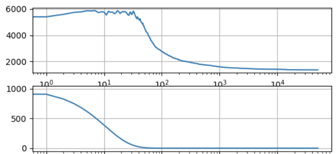
The figure below shows the progress of 100 x 50000 optimization steps in a more complex design (top row is netlength, bottom row is temperatere).  You can see that some increase of netlength takes place while the temperature is high. This is expected behavior and shows that the algorithm works as intended.

Since simulated annealing is prone get stuck in local optima, initial optimization is attempted on 20 candidates with different random seeds and detailed optimization is performed only on the best candidate. There are certainly many ways to improve the optimization further, but for now it is good enough. Run time is 1-10 minutes, depending on design size.

Optimized cell placement for the counter example is shown below.

Final length: 163
X       0      1      2      3      4      5      6
Y
0      IO     IO     IO     IO     IO     IO     IO
1   EMPTY  EMPTY  EMPTY  EMPTY    NOT    NOT  EMPTY
2   EMPTY  EMPTY    NOT  EMPTY    NOT    NOT  EMPTY
3   EMPTY    NOT    NOT  EMPTY    NOT    NOT  EMPTY
4   EMPTY    NOT    NOT    NOT    NOT    NOT  EMPTY
5   EMPTY    NOT    NOT    NOT    NOT    NOT  EMPTY
6     NOT    NOT    NOT    NOT    NOT    NOT    NOT
7     NOT    NOT    NOT    NOT    NOT    NOT    NOT
8     NOT    NOT    NOT    NOT    NOT    NOT    NOT
9   EMPTY    NOT    NOT    NOT    NOT    NOT    NOT
10  EMPTY  EMPTY    NOT    NOT    NOT    NOT    NOT
11  EMPTY  EMPTY    NOT    NOT    NOT    NOT    NOT
12  EMPTY  EMPTY  EMPTY    NOT    NOT    NOT    NOT
13  EMPTY  EMPTY  EMPTY    NOT    NOT    NOT  EMPTY
14  EMPTY  EMPTY  EMPTY  EMPTY    NOT    NOT  EMPTY
15  EMPTY  EMPTY  EMPTY  EMPTY  EMPTY  EMPTY  EMPTY

Due to the way the optimization criteria are defined, the cells tend to gravitate toward a common center of mass.

X                  0                  1                   2                   3                   4                   5                  6
Y
0              [VCC]              [clk]               [rst]           [count.0]           [count.1]           [count.2]              [GND]
1                 []                 []                  []                  []  [count.1, X12bX2o]  [X10bX2o, count.2]                 []
2                 []                 []  [count.0, X11bX2o]                  []  [X12bX2o, count.1]      [clk, X10bX2o]                 []
3                 []      [clk, X11bCI]  [X11bX2o, count.0]                  []      [clk, X12bX2o]  [count.2, X10bX2o]                 []
4                 []  [X11bCI, X11bX1o]      [clk, X11bX2o]  [X12bX1o, count.1]    [X12DI, X12aX2o]    [X12aX2o, X12DI]                 []
5                 []   [X11DI, X11bX1o]  [X11bX1o, count.0]   [X12bCI, X12bX1o]    [X12DI, X12bX1o]    [X12CI, X12aX2o]                 []
6   [X11DI, X11aX2o]   [X11aX1o, X11DI]        [count.0, 4]       [clk, X12bCI]    [X12aX1o, X12DI]        [clk, X12CI]   [X10aX2o, X10DI]
7   [X11aX2o, X11DI]  [X11aCI, X11aX1o]        [4, X11aX1o]        [count.0, 9]   [X12aCI, X12aX1o]     [X12CI, X12aCI]   [X10DI, X10aX2o]
8   [X11CI, X11aX2o]    [X11CI, X11aCI]            [rst, 4]        [count.1, 9]       [10, X12aX1o]        [clk, X10CI]   [X10CI, X10aX2o]
9                 []       [clk, X11CI]        [count.0, 1]             [9, 10]        [count.1, 2]       [clk, X10bCI]    [X10CI, X10aCI]
10                []                 []              [1, 7]           [rst, 10]              [2, 7]   [X10bCI, X10bX1o]  [X10aCI, X10aX1o]
11                []                 []              [1, 5]             [5, 10]              [2, 5]    [X10DI, X10bX1o]   [X10aX1o, X10DI]
12                []                 []                  []            [rst, 8]              [5, 6]  [X10bX1o, count.2]       [8, X10aX1o]
13                []                 []                  []              [7, 8]              [6, 8]        [count.2, 6]                 []
14                []                 []                  []                  []              [3, 7]        [count.2, 3]                 []
15                []                 []                  []                  []                  []                  []                 []

Net assignments are show above. One can observe that cells with common nets are located close together. The complex net names are the results of recursively breaking down the synthesized cells into physical ones.

The placement and optimization is implemented in the CellArray class of  PCBPlace.py