 Anand Uthaman
A multitude of use cases needs AI along with depth information for meaningful deployment in real-world scenarios. Let's dive deep into each mentioned solution, to experience the possibilities of Depth AI in various domains. The technical milestones and progress sequence of each solution would unfold in the "Project Log" section.
Consolidated Project Demo
Solution #1: ADAS - Collision Avoidance System on Indian Cars
India accounts for only 1% of total vehicles in the world. However, World Bank’s survey reports 11% of global road death happens in India, exposing the dire need to enhance road safety. Most of the developing countries like India pose a set of challenges, unique on their own. These include chaotic traffic, outdated vehicles, lack of pedestrian lanes and zebra crossings, animals crossing the road, and the like. Needless to say, most vehicles don't have advanced driver-assist features nor can they afford to upgrade the car for better safety.
Against this backdrop, this solution aims to augment even the least expensive cars in India with an ultra-cheap ADAS Level 0, i.e. collision avoidance and smart surround-view. Modern cars with a forward-collision warning (FCW) system or autonomous emergency braking (AEB) are very expensive, but we can augment such functions on old cars, at a low cost.
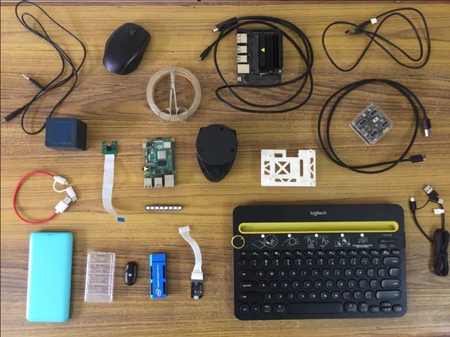
The idea is to use a battery-powered Pi connected with a LIDAR, Pi Cam, LED SHIM, and NCS 2, mounted on the car bonnet to perceive frontal objects with their depth and direction. This not only enables a forward-collision warning system but also driver assistance alerts about traffic signs or pedestrians, walking along the roadside, or crossing the road.
To build a non-blocking system flow, a modular architecture is employed wherein, each independent node is dependent on different hardware components. i.e., the "object detection" node uses Movidius for inference, whereas the "distance estimation" node takes LIDAR data as input, while the "Alert" module signals to Pimoroni Blinkt and the speaker. The modules are communicated via MQTT messages on respective topics.
Architecture Diagram

The time synchronization module takes care of the "data relevance factor" for Sensor Fusion. For ADAS, the location of detected objects by 'Node 1' may change, as the objects move. Thus, the distance estimate to the bounding box could go wrong after 2-3 seconds (while the message can remain in the MQTT queue). In order to synchronize, current time = 60*minutes + seconds is appended to the message (to ignore lagged messages at receiving end).
Watch the gadget plying the Indian Roads, giving driver-assist...
Read more »


 Jazmín Peña
 Johanna Shi
 Jerry Isdale
Great..
hats off ..