A servo motor is a motor that maintains a given position, but how does it get to that position?

A normal servomotor only receives the final position by PWM and always goes as fast as it can to that point. A smart servo motor, on the other hand, usually receives a command that tells it the end position and how fast it has to reach that position, at which point the smart servo motor starts to calculate the path to the end position. There are several ways to trace the route, those are the motion curves.

LINEAR

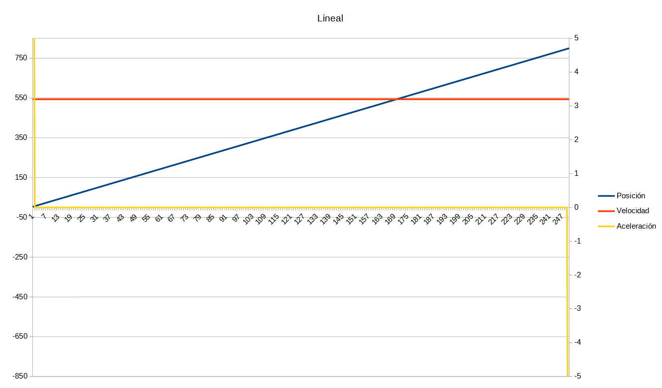
It is the most basic, the space is divided by the time you have and a constant velocity is calculated. The problem is that it proposes an almost infinite initial and final acceleration. This kick of acceleration causes great mechanical wear in motor and gears and strong vibrations by the accelerations.

In the following picture it can be clearly seen, left axis corresponds to position and acceleration, while the right axis is velocity:

TRAPEZOIDAL

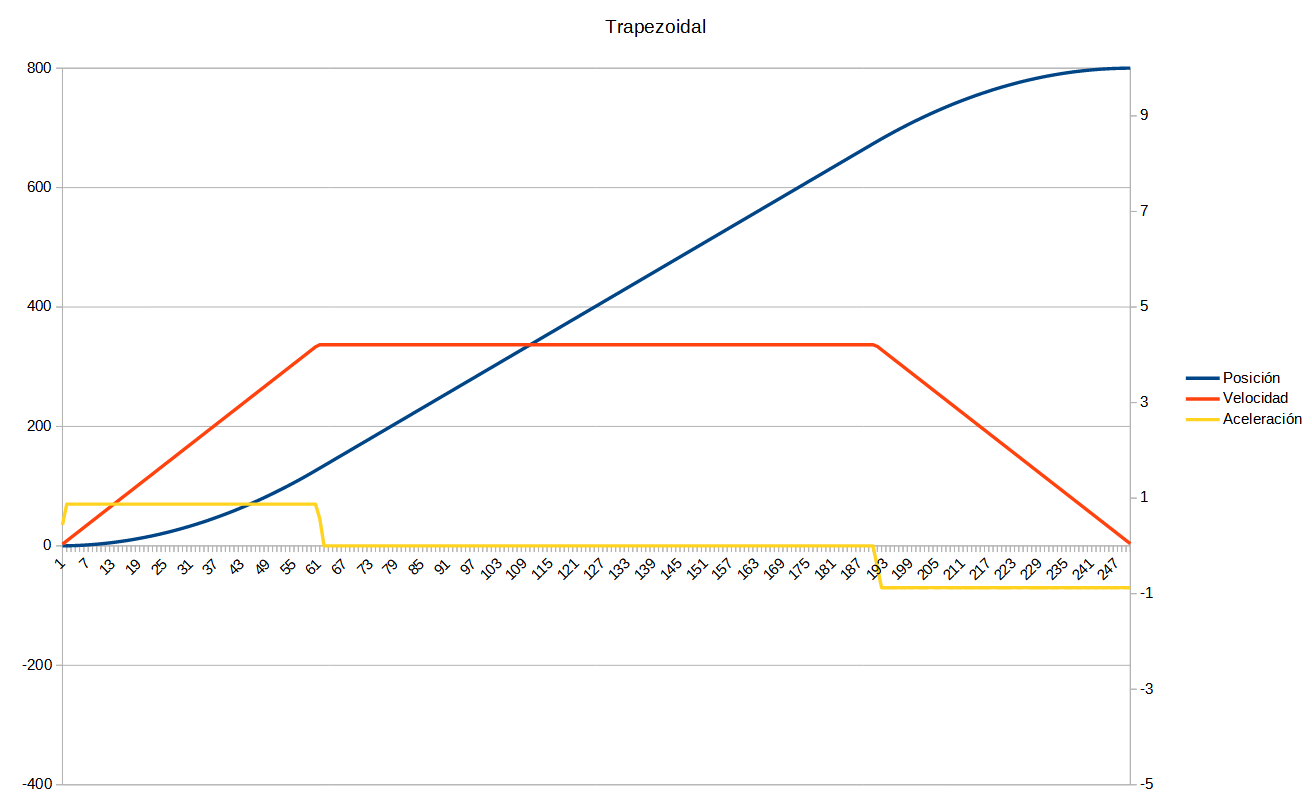
To reduce the acceleration kick, a profile with a constant maximum acceleration is created. This generates an initial acceleration ramp, a constant velocity section and a final deceleration section. This is the only motion curve with the above that manufacturers offer. The problem with it is that it still generates vibrations from abrupt changes in acceleration. It is smoother than the previous profile, but it still has vibrations.

S-CURVE

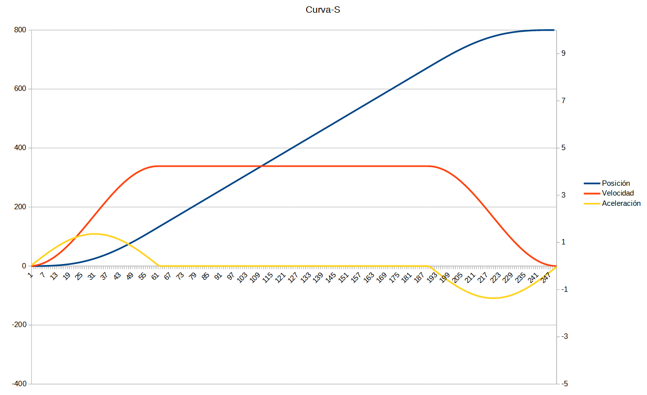
This motion curve is not offered by manufacturers, but is offered by LibreServo. This motion curve is intended to completely eliminate any acceleration kick. This motion curve is specific to make a clean acceleration transition without jumps as seen in the graphs.

HERMITIC CURVE

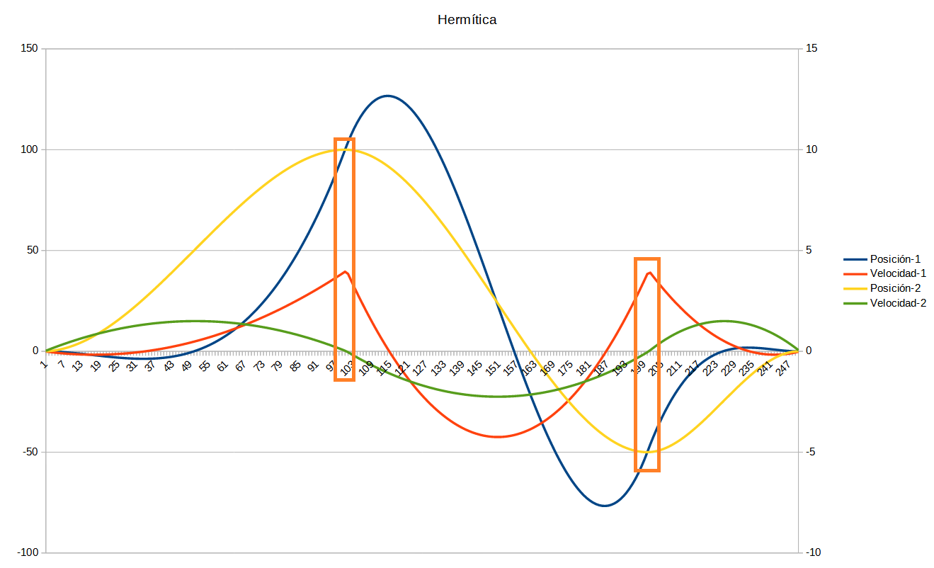
This motion curve is again unique to LibreServo. All other curves presuppose starting from a standstill and ending at a standstill, this is the only curve that allows to start and end the movement starting or ending at a given velocity. This is indispensable in situations where we want to end a movement or modify it in the middle of a run, for example, if we detect a possible fall, a possible error or some danger. In addition, it is perfect for passing through different marked points at different speeds, LibreServo will take care of executing the curve. This curve continues a movement, but not the acceleration it already had, so it can generate vibrations.

In the following picture we see two different paths. In both we start from 0, go through 100, through -50 and back to zero, but in the first path the velocity at each point is always indicated to be zero, while in the second path at the intermediate points the velocity will be 4.

Text extracted from: https://www.libreservo.com/en/articulo/motion-curves