 Simon Trendel
We are a student team from Munich, Germany. Our goal is to make Roboy balance and walk. For this we need accurate tracking. We decided to replicate HTC lighthouse tracking for our purposes and in November 2016 a fascinating journey began.
Checkout this excellent review on the HTC lighthouse tracking system.
At first we tried decoding the signals from the sensors using Intel Edison and MKR1000, which in case of the Edison turned out to be impossible and in case of the MKR was limited to a small amount of sensors. For the Edison the hardware interrupts were not handled fast enough. This is due to a threaded interrupt system. We also tried using the MCU, which wasn't fit for the job eaither.
The MKR was simply overwhelmed by all the interrupts.
We disassembled one of the HTC vive controllers for getting our hands on those sensors. We noticed the HTC controllers were using an ICE fgpa. So we thought if they use it, there must be a reason.
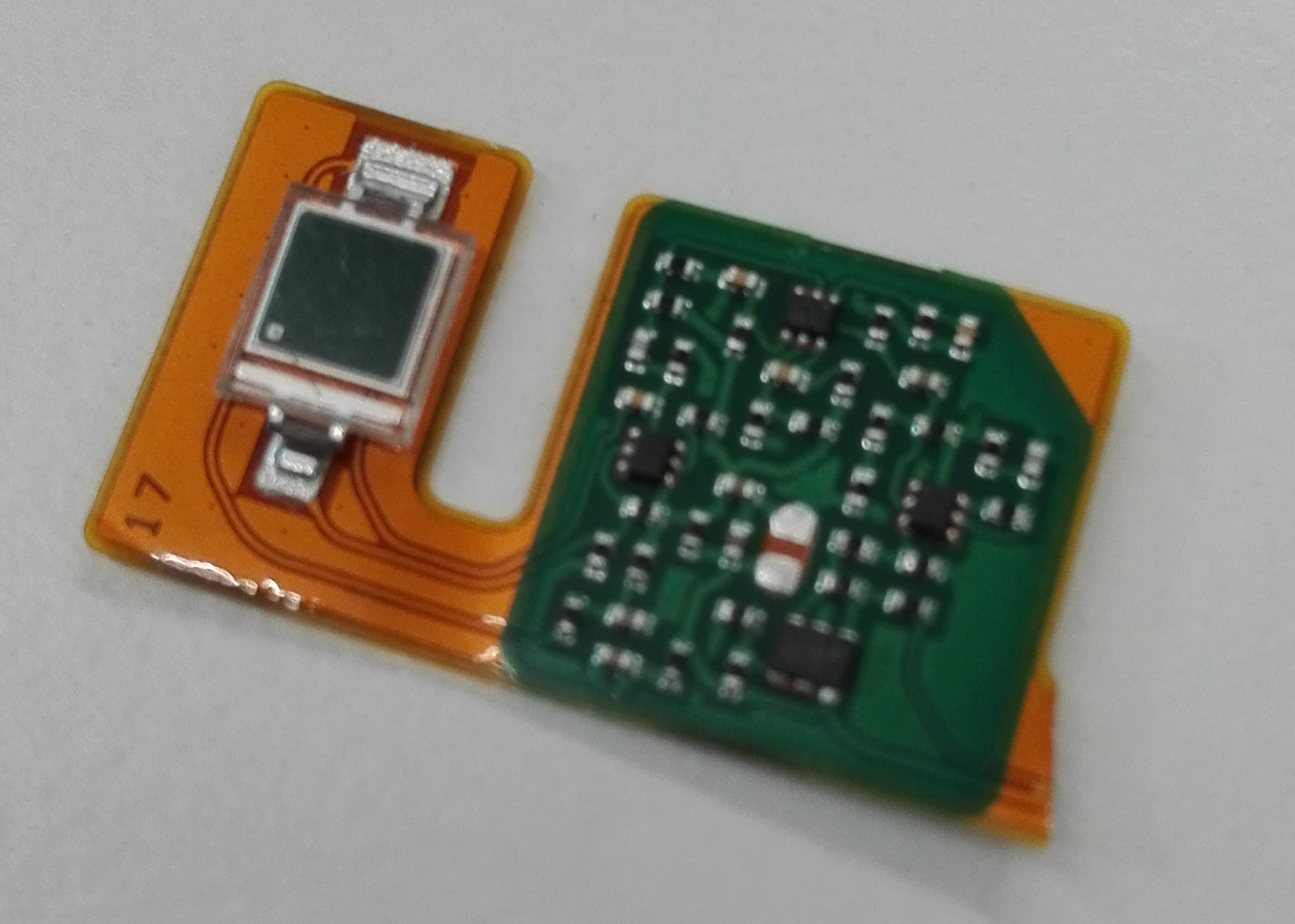
Then soldered VCC, GND and Signal copper cables (0.1 mm), using enough flux. And covert the sensor with a bit of glue to protect it from accidental damage.

In the previous prototype we were routing all signal cables coming from the sensors in parallel. This turned out to be a bad idea. Because of induction the signals pollute each other. In the vive controller, they deal with it by isolating the signal with VCC and GND. So thats what we are also doing.
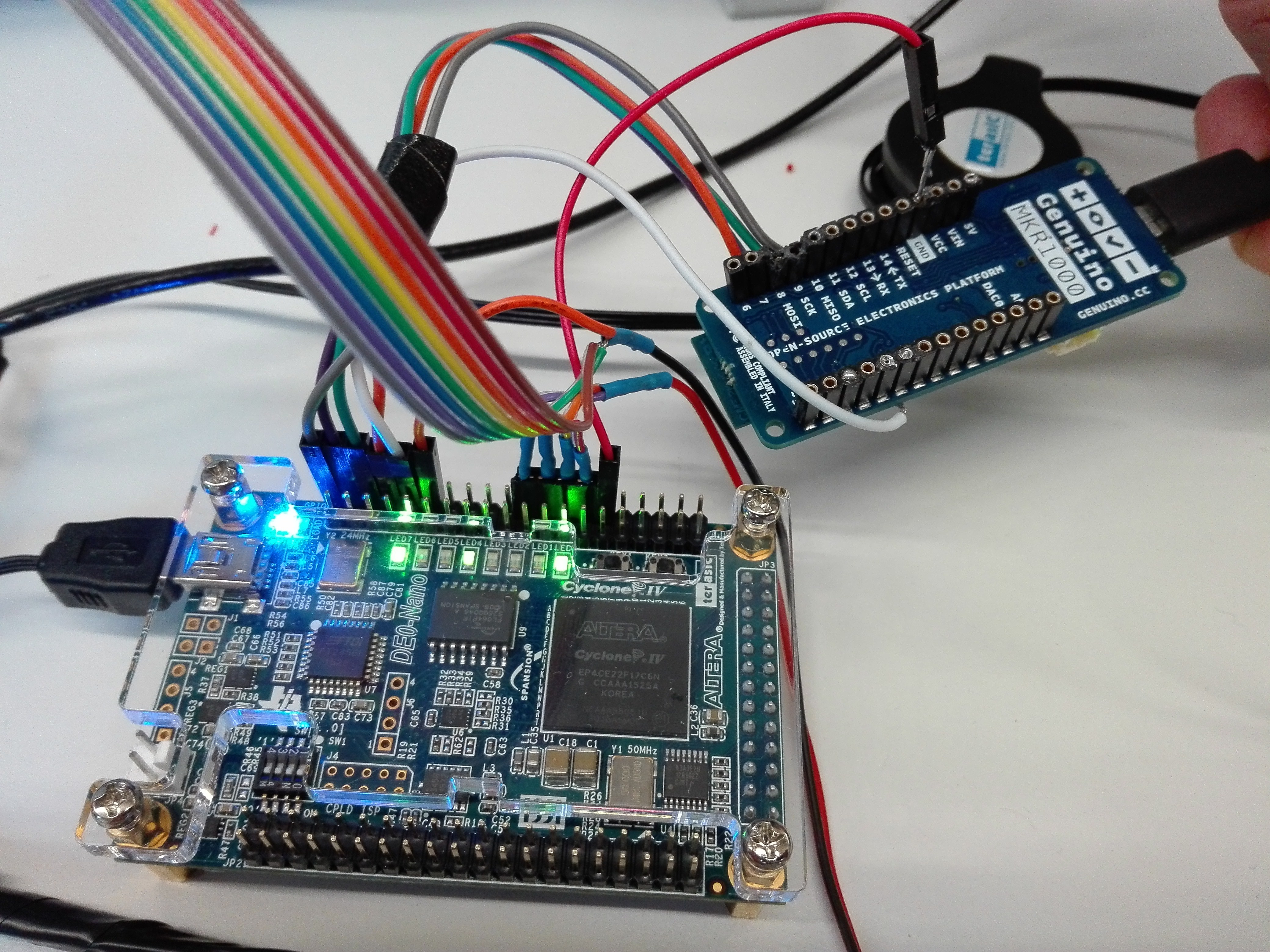
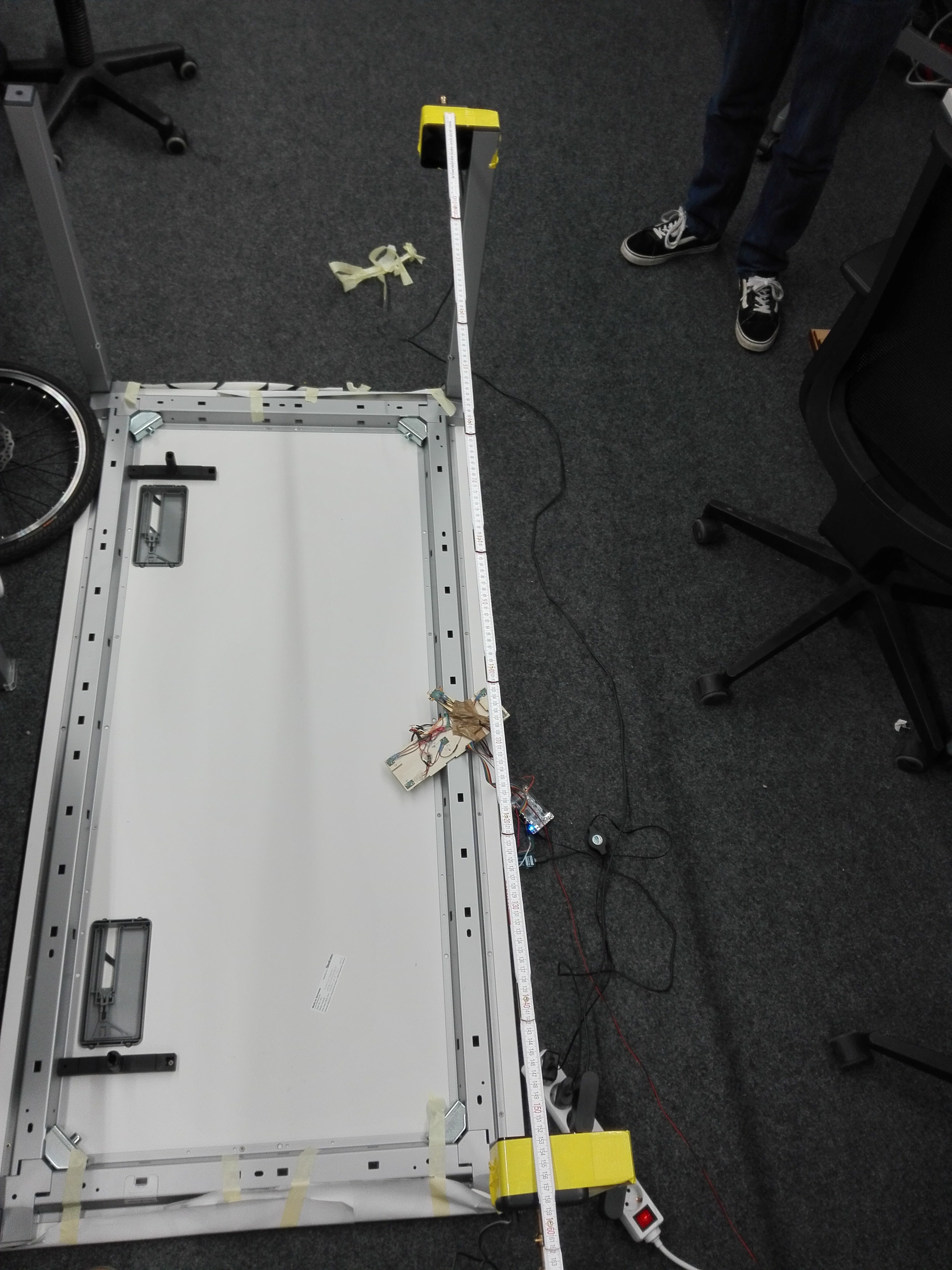
In the following picture you can see the complete setup:
- The custom object, with 4 sensors
- The de0 nano FPGA
- The MKR1000
[Note: This is the old setup. New updated setup is described in section 7.]
Notice that there are only 4 sensor signal cabels (grey, blue, yellow, red). The other cables are VCC (purple, orange) and GND (green, brown).
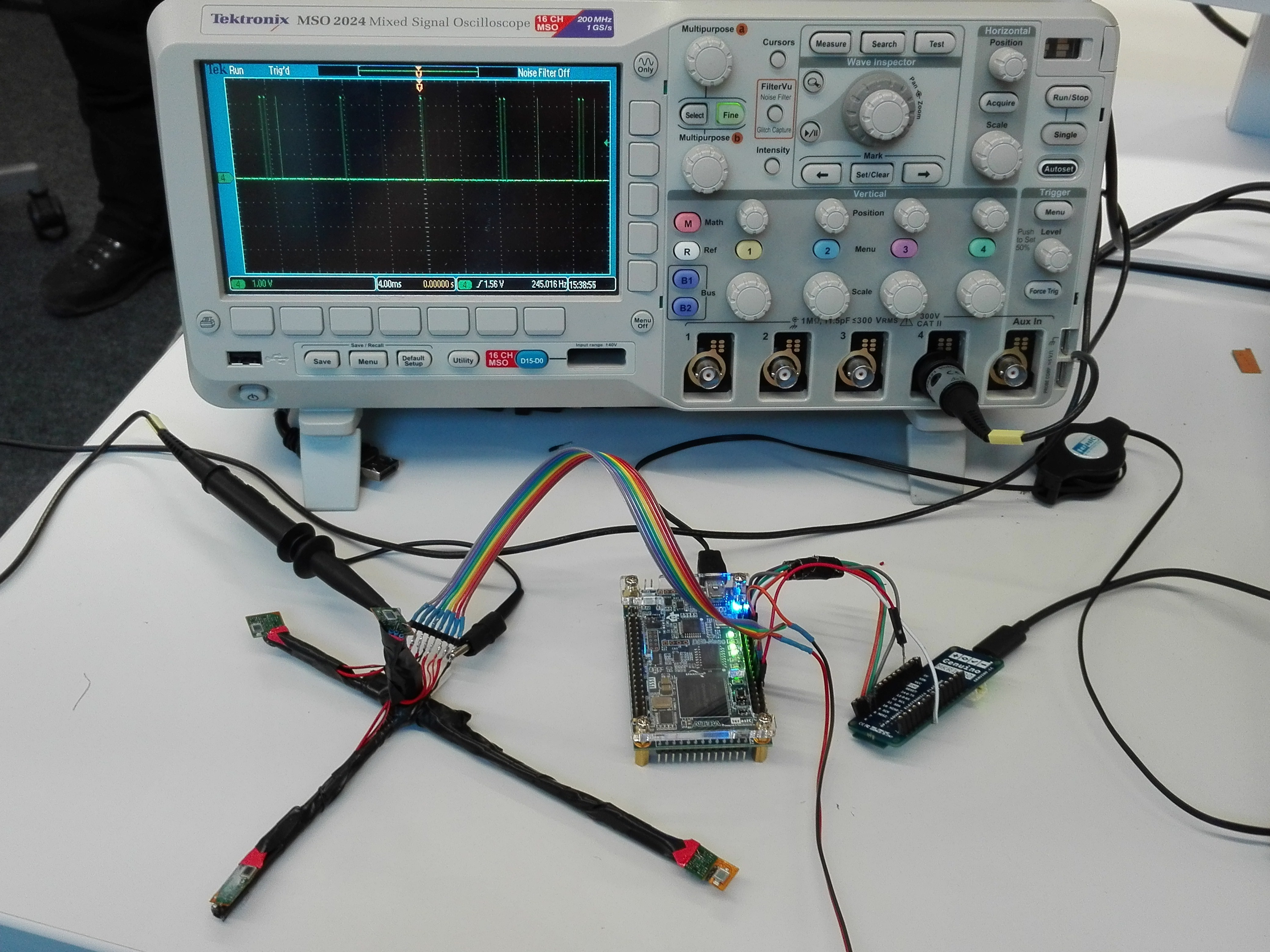
The connection to the MKR is via SPI, where the MKR acts as the Master. An additional pin to the MKR notifies the MKR, when there is new data available. This triggers the SPI transfer.
Our vive tracking consists of a couple of modules:
- Decoding the sensor signals and calculating the sweep durations (this is done on the fpga)
- Transmitting the sensor values via SPI to the MKR1000
- Transmitting the sensor values wirelessly via UDP to the host
- Triangulation of the ligthhouse rays
- Distance Estimation wrt a calibrated object
- Relative Pose correction using a calibrated object
1. Decoding sensor signals
[Note: This is the old decoder. New updated decoder is described in section 7.]
On the de0 we are using a PLL to get a 1MHz (1us) clock
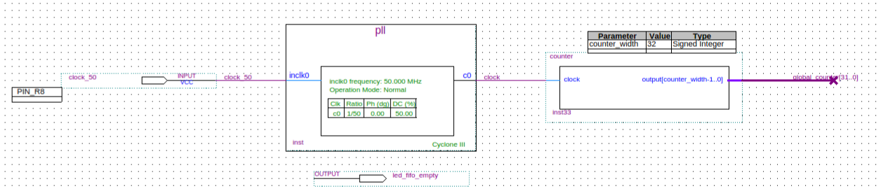
Then we feed the sensor signals to one of these lighthouse modules
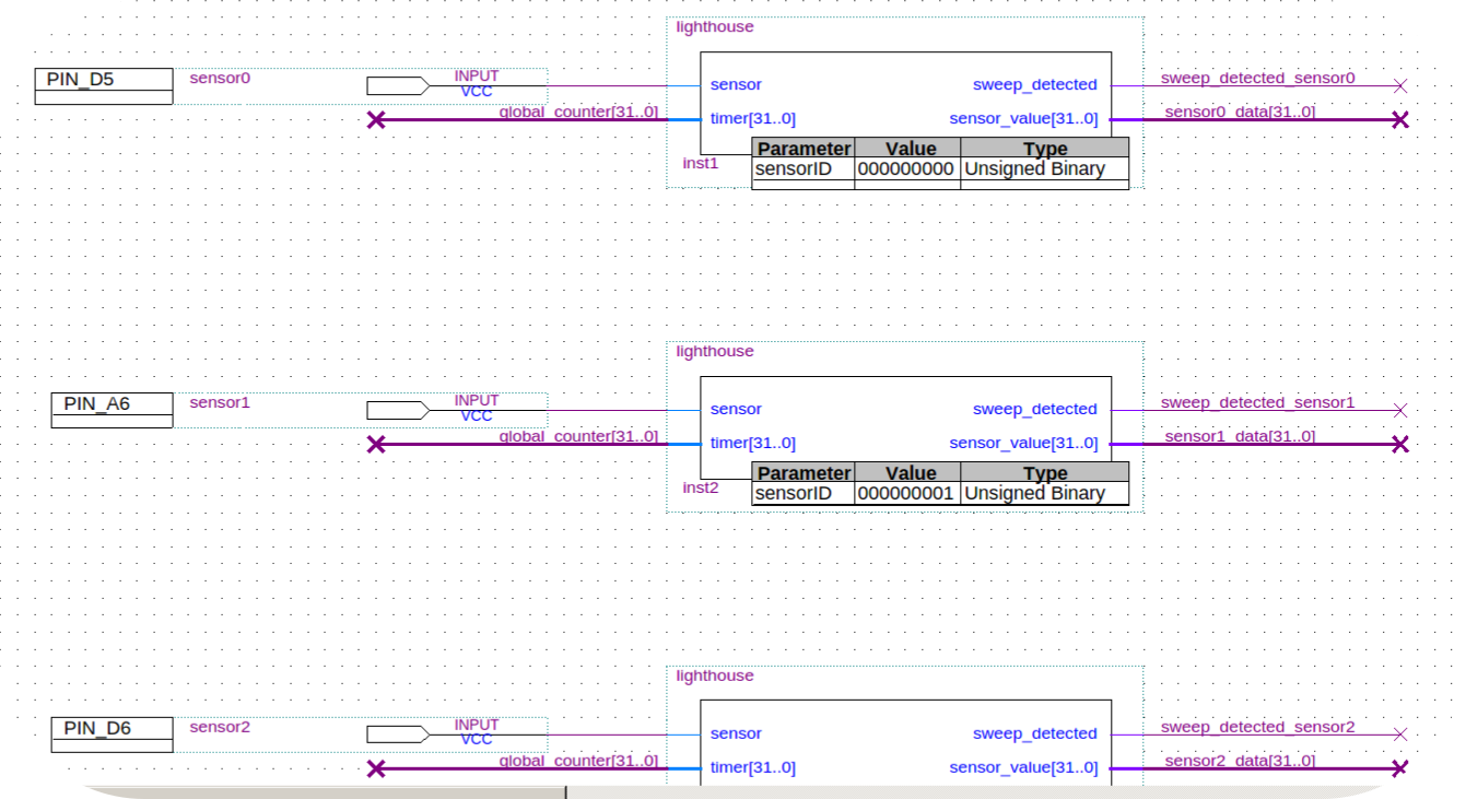
The spi module looks like this
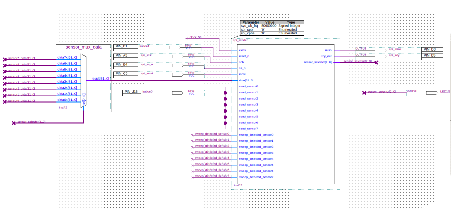
2. Transmitting the sensor signals via SPI
[Note: This is the old data format. New data format is described in section 7.]
The MKR acts a the SPI Master. Whenever there is new data available (ie when the fpga decoded a valid sweep), it notifies the MKR via an extra pin. The MKR then starts downloading a 32 bitfield, which encodes the data in the following way:
- bits 31 - 13: sweep duration (in micro seconds)
- bit 12: valid sweep
- bit 11: data
- bit 10: rotor
- bit 9: ligthhouse
- bits 8-0: sensor id
3. Transmitting the 32-bitfield via UDP
The host listens to UDP broadcast messages. We are using google protobuffer for the custom messages. When the host receives a trackedObjectConfig message, it opens sockets for the sensor and logging messages and sends the respective ports via a commandConfig message to the MKR. The MKR is waiting for this message and once received, starts sending the sensor values augmented with a milliseconds timestamp.
This sort of infrastructure is very convenient once you start using many tracked objects. You just turn the thing on and the tracking is initiated. We implemented a yaml reader, which saves and reads information about an object (eg the relative sensor locations on the object, or a mesh to be used with it...).
4. Triangulation of the lighthouse rays
The rays are calculated using the following illustration: EDIT (THIS IS INCORRECT AND WAS REPLACED BY SPHERICAL COORDINATES)
EDIT EDIT (math is fine, checkout log 6 for update)

Once you calculated the rays for both lighthouses, you can triangulate to get the sensor positions. For the triangulation to be valid, you need to know the transformation between the lighthouses. When you have no calibrated object you can start by placing the lighthouses at a know configuration to each other.
In our case we used a table:
Then you can calibrate the unknown object (ie estimating the realtive sensor locations on the object). This is done by measuring the triangulated sensor locations for 30 seconds and taking the mean positions. The mean positions are the absolute sensor positions (in our world_vive fram), so we define an arbitrary origin by taking the average positions of the sensors. We then define the relative sensor locations wrt to this origin and save them to a yaml file. Next time this object comes online, you have its relative sensor locations ready.
5. Distance Estimation wrt a calibrated object
You can use this relative distance to estimate the distance of each sensor to a single lighthouse (so without triangulation).
Regarding the distance estimation we used this paper.
6. Relative pose correction
With the relative sensor locations wrt to each ligthhouse we can estimate the relative lighthouse pose.
The relative lighthouse poses can be estimated using levenberg-marquardt and minimizing the squared distances from 5. It looks like this:
7. July 2017 Update
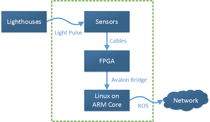
Most of the FPGA code was changed in July 2017. The new architecture doesn't need the MKR1000 board. We only use the resources of the DE0-Nano board: the FPGA and the ARM core. The sensor inputs are still processed on the FPGA. The results are transferred to the ARM code via the built in Avalon bridge. Ubuntu 16 is running on that core and sends the data to the network using ROS. Data flow looks like this:
7.2 Lighthouse signals
Both lighthouses are synchronized and follow a specific protocol. Every second, there are 120 phases. Each phase has the duration of 8333
μs (microseconds) and contains exactly three light pulses. First, each
lighthouse sends a long pulse. Then, one of the lighthouses sweeps the
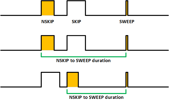
room with laser (short pulse). There types of light pulses are:
- SKIP: the lighthouse sending this pulse will not sweep the room with laser (longest pulse)
- NSKIP (not skip): the lighthouse will sweep the room with laser (long pulse)
- SWEEP: laser sweeps the room on x or y axis (short pulse)
The measured duration between the start-of-the-last-NSKIP and start-of-the-last-SWEEP
defines the angle from the lighthouse to the sensor. By combining angle
data from both lighthouses and both axes, the position of the sensor
can be calculated as described above. Examples of phases and pulse types:
7.2 New VHDL core for signal processing
We made some changes to the signal processing cores. The PLL that was slowing down the clock was removed. Original 50 MHz clock is now used and provides more accurate results.
Each core is a state machine with two main states: HIGH and LOW. In general, the
states correspond to the value of the input sensor signal. To avoid
noise, additional filtering is done. The internal state will change only
when the input signal changes and stays constant for some time.
The module has several internal counters to measure the duration of
pulses. Outputs are updated every time a SWEEP was detected. It is
possible to find out which of the two lighthouses was sweeping the room
depending on the duration between two NSKIP pulses. If this duration is
approximately equal to the phase duration (8333 μs), the active
lighthouse didn't change. Otherwise the active lighthouse has changed.
All SKIP pulses are completely ignored.
7.3 New data format
The data format was changed. Data is send over the network as ROS messages. Each ROS message that is sent contains N 32-bit data values, one value for each of the N sensors. Note that there are no explicit sensor IDs anymore. The first value corresponds to the first sensor and so on. Each data value has the following format:
| Bit position | Meaning | Comment |
| 31 (MSB) | Lighthouse ID | The sensor is illuminated by two different lighthouses. This ID indicates which lighthouse has just swept the room with laser. |
| 30 | Sweep Axis | Indicates which axis (x or y) was swept. |
| 29 | Valid | This flag is set if data for this sensor is valid. This is the case if duration is between 300 and 8000 microseconds. |
| 28 to 0 | Duration | Duration between start-of-the-last-NSKIP and start-of-the-last-SWEEP (unsigned number). Divide this value by 50 to get microseconds. |