We were going to start shifting over to a site more oriented toward learning calculus (rather than our musings about how we are doing the development) but we thought we would put up just one more idea here first to get some feedback. It's a little preliminary, so we're not posting the models yet- but we would love some thoughts on the ideas!
Our PID controller model is really a model of a two-dimensional system- a signal and its variation with time. We made it a three-dimensional piece by showing the derivative and integral of the system to show how each of these contributes to the final solution on a PID controller. But in some ways, you could do that with multiple lines on a traditional graph.
So, instead, we said: what if you could model a truly 3D system, where you are showing how, for instance, two things are varying with time? We hunted around a bit and asked some folks for good candidate equations, and our mathematician friend Niles Ritter suggested we look into the predator-prey equations.
These equations model how two populations, one of which eats the other one, vary over time. Populations will swell and contract as first the prey have a population boom and then the predators catch up and overtake. (Often the example used is rabbits and foxes, if this is starting to sound dimly familiar!)
The equations for this are called the Lotka-Volterra equations, and they come up in a variety of other contexts as well. Their basic form is a pair of equations like this, where x = predators, y = prey, t = time, and a, b, c and d are constants:
dx/dt = ax – bxy
dy/dt = cxy – dy
We approximated dx/dt in the most simple-minded way possible:
dx/dt = x at the current time – x at the previous time/time difference
creating a standard time step and solving for x and y at each time step by using x and y at the previous time step. There are many more sophisticated ways of doing this, but we wanted something simple we could toss into OpenSCAD and mess with.
It turns out (see the Wikipedia article linked above) that if a=2/3, b=4/3, c=d=1, that there is stable oscillatory behavior of the two populations. They grow and sink together. (Another stable state is that both populations go extinct after some wild variation, but what fun is that?)
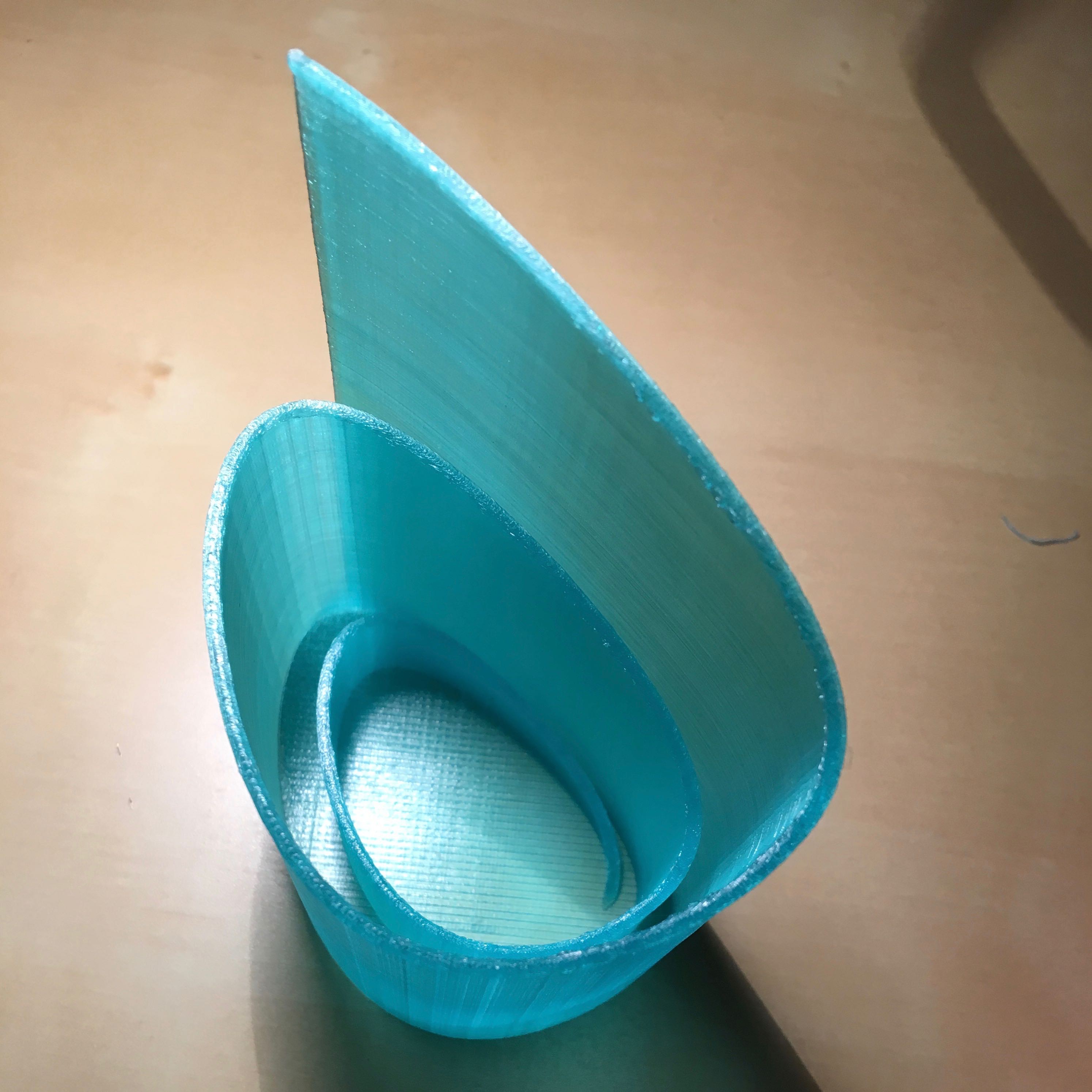
Our first attempt to plot the three-dimensionally, messing around a bit with a,b,c,d and the starting values for the population, had time coming up from the platform, and looked like this. The numbers of rabbits and foxes are the x and y axes respectively, and time is coming up toward you.
 Expanding Lotke-Volterra equations solution
However, the particular set of equations we were trying out were not supposed to expand like that (although it looked cool.) Joan remembered her graduate school math and realized we needed to use either a smaller time step size or a more sophisticated way of modeling the derivative or both (we went with a smaller time step.)
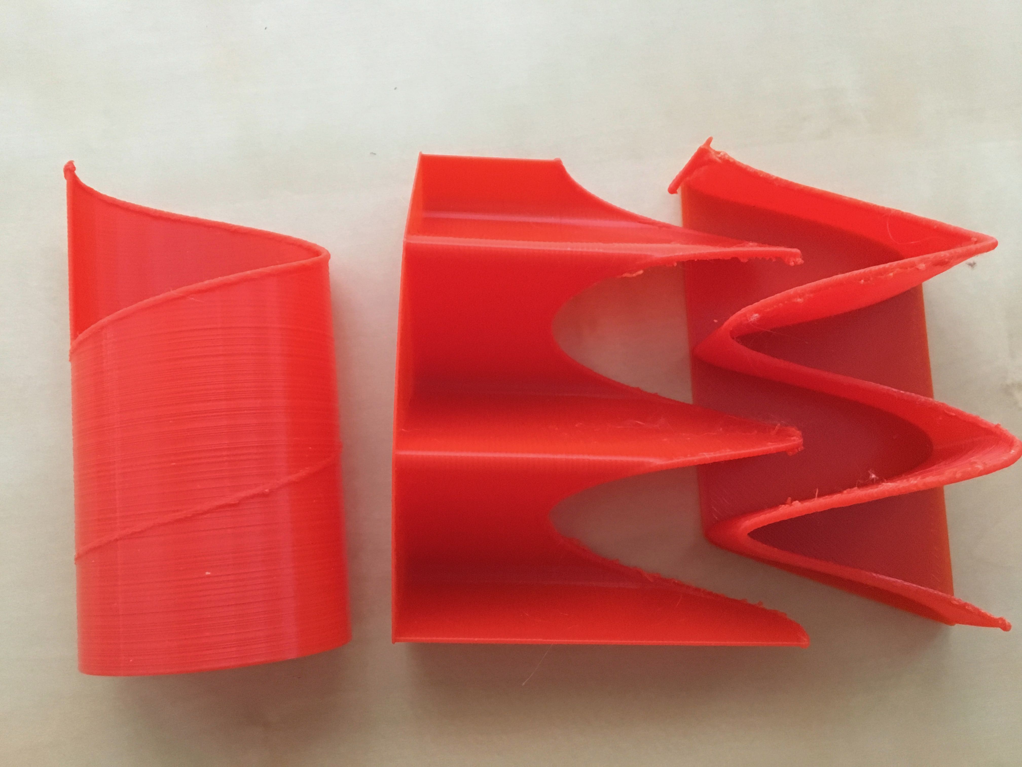
Rich also decided to try printing with different axes “up” in the print. So here is what the correct version looks like, printed with time going toward the top of the the picture but with each one printed with a different pair of axes on the build platform of the 3D printer:
 Three versions of the visualization, printed with different axis "up" during printing.
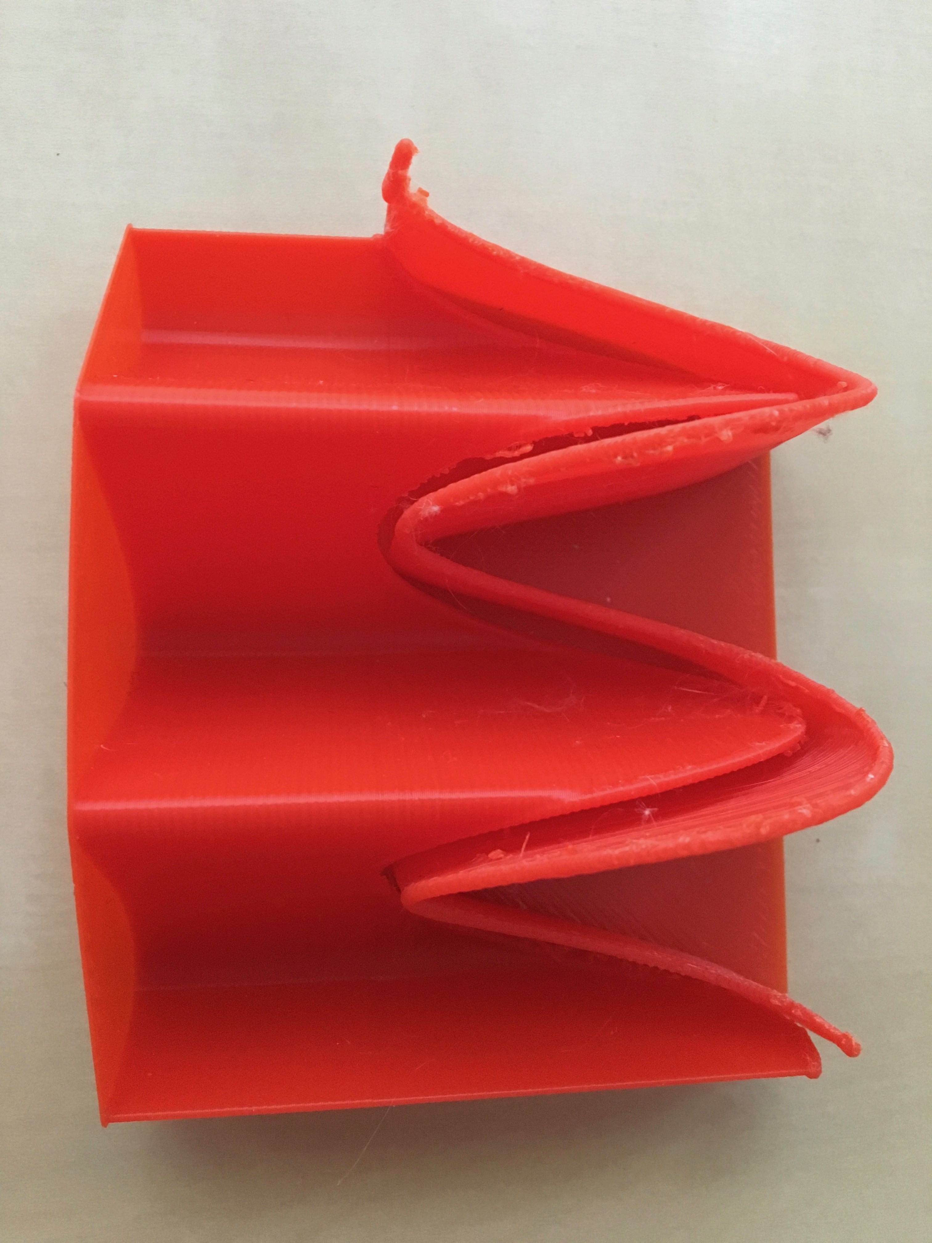
It's also cool to note that two of these fit into each other. The one above that looks like a toilet paper tube is the equivalent of the one that expanded, but with the numerical instability corrected.

Two versions fit into each other
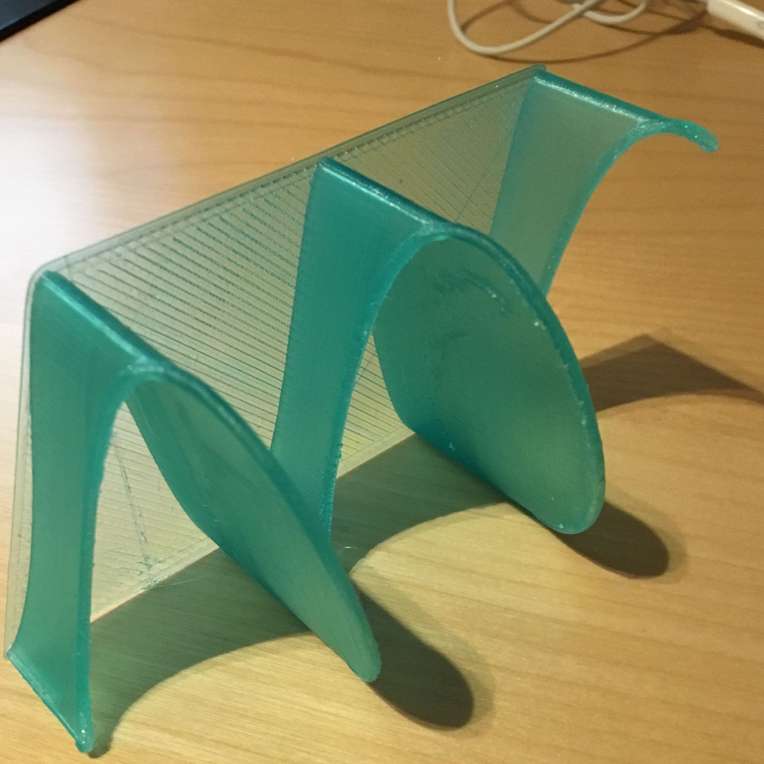
The version we find the most explanatory is the one below. Imagine the line in space describing the rabbits, foxes and time running along the top surface of this, making a spiral. Time goes left to right, rabbits are in the vertical axis, and foxes are toward you in this orientation.

Best orientation predator prey visualization
And if you look straight back through it, you'll see a sinusoid - the projection of the prey varying over time. Looking at 90 degrees gives you the variation of the predators over time.
There are a lot of "famous equations" out there that happen to govern a lot of interesting phenomena, and we want to try out some of the more stable ones once we get the kinks out of this one. We're not putting out the model for this one just yet, because it's still got some numerical instabilities and issues. But we wanted to let you see our very latest cool stuff before the deadline closes in! We are looking into various options for a long-term home for these models and the math, so stay tuned about where these later explorations wind up living.
 Joan Horvath
Discussions
Become a Hackaday.io Member
Create an account to leave a comment. Already have an account? Log In.