 Marcel van Kervinck
Pipelining basics
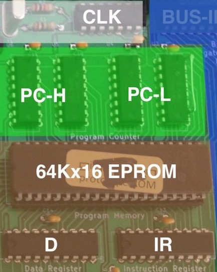
Our computer uses simple pipelining: while the current instruction is stable in the IR and D registers and executing, the next instruction is already being fetched from program memory.
This makes high speeds possible, but comes with an artefact: when a branch is executing, the instruction immediately behind the branch has already been fetched. This instruction will be executed before the branch takes effect and we continue from the new program location. Or worded more properly: the effect of branches is always delayed by 1 clock cycle.
When you don't want to think about these spurious instructions you just place a nop (no-operation) behind every branch instruction. Well, our instruction set doesn't have an explicit nop, but ld ac will do. My disassembler even shows that instruction as a nop. The Fibonacci program uses this all over:
address
|    encoding
|    |     instruction
|    |     |    operands
|    |     |    |
V    V     V    V
0000 0000  ld   $00
0001 c200  st   [$00]
0002 0001  ld   $01
0003 fc0a  bra  $0a
0004 0200  nop
0005 0100  ld   [$00]
0006 c202  st   [$02]
0007 0101  ld   [$01]
0008 c200  st   [$00]
0009 8102  adda [$02]
000a c201  st   [$01]
000b 1a00  ld   ac,out
000c f405  bge  $05
000d 0200  nop
000e fc00  bra  $00
000f 0200  nop
If you don't want to waste those cycles, usually you can let the extra slot do something useful instead. There are two common folding methods. The first is jumping to a position one step ahead of where you want to go, and copy the missed instruction after the branch instruction. In the example above, look at the branch on address $000e, it can be rewritten as follows:
000e fc01  bra  $01   # was: bra $00
000f 0000  ld   $00   # instruction on address 0
The second method is to exchange the branch with the previous instruction. Look for example at the branch on address $0003. The snippet can be rewritten as follows:
0002 0001  bra  $0a   # was: ld   $01
0003 fc0a  ld   $01   # was: bra  $0a
0004 0200  nop        # will not be executed and can be removed
One of these folding methods is often possible, but not always. Needless to say, applying this throughout can lead to code that is both very fast and very difficult to follow. Here is a delay loop that runs for 13 cycles:
address
|    encoding
|    |     instruction
|    |     |    operands
|    |     |    |
V    V     V    V
0125 0005  ld   $05 # load 5 into AC
0126 ec26  bne  $26 # jump to $0126 if AC not equal to 0
0127 a001  suba $01 # decrement AC by 1
This looks like nonsense: the branch is jumping to its own address and the countdown is in the instruction behind. But due to the pipelining this is just how it works.
Advanced pipelining: lookup tables
The mind really boggles when the extra instruction is a branch itself. But there is a useful application for that: the single-instruction subroutine, a technique to implement efficient inline lookup tables.
Here we jump to an address that depends on a register value. Then immediately following we put another branch instruction to where we want to continue. On the target location of the first branch we now have room for "subroutines" that can execute exactly one instruction (typically loading a value). These subroutines don't need to be followed by a return sequence, because the caller conveniently just provided that... With this trick we can make compact and fast lookup tables. The LED sequencer from yesterday's video uses this to implement a state machine:
address
|    encoding
|    |     instruction
|    |     |    operands
|    |     |    |
V    V     V    V
0105 0009  ld   $09    # Start of lookup table (we stay in the same code page $0100)
0106 8111  adda [$11]  # Add current state to it (a value from 0-15)
0107 fe00  bra  ac     # "Jump subroutine"
0108 fc19  bra  $19    # "Return" !!!
0109 0010  ld   $10    # table[0] Exactly one of these is executed
010a 002f  ld   $2f    # table[1]
010b 0037  ld   $37    # table[2]
010c 0047  ld   $47    # table[3]
010d 0053  ld   $53    # table[4]
010e 0063  ld   $63    # table[5]
010f 0071  ld   $71    # table[6]
0110 0081  ld   $81    # table[7]
0111 0090  ld   $90    # table[8]
0112 00a0  ld   $a0    # table[9]
0113 00b1  ld   $b1    # table[10]
0114 00c2  ld   $c2    # table[11]
0115 00d4  ld   $d4    # table[12]
0116 00e8  ld   $e8    # table[13]
0117 00f4  ld   $f4    # table[14]
0118 00a2  ld   $a2    # table[15]
0119 c207  st   [$07]  # Program continues here
At runtime 6 instructions get executed: ld, adda, bra, bra, ld, st
(Note: The values in this example are not important. If interested: the high 4 bits are the new state in the state machine, and the low 4 bits are the 4 LED outputs. This snippet of code implements the startup sequence and moving scanner lights from the video.)
Hyper advanced pipelining: the ternary operator
The pipeline gives a nice idiom for a ternary operator. With that I mean constructs like these:
V = A if C else B       # Python
V = C ? A : B           # C
if C then V=A else V=B  # BASIC
The simple way to do this is as follows:
        ld  [C]
        beq done
        ld  [B]
        ld  [A]
done:   st  [V]
The folding methods are already applied. In the false case (C == 0), B gets stored and this takes 4 cycles. In the true case B gets loaded first but is then replaced with A, which gets stored. This takes 5 cycles.
If you are in a time-critical part, such as in the video loop of this computer, this timing difference is quite annoying because we have to keep each path exactly in sync. The naive way to make both branches equally fast is something like this:
        ld  [C]
        beq label
        ld  [B]
        bra done
        ld  [A]
label:  nop
        nop
done:   st  [V]
Now each path takes 6 cycles and doesn't mess up our timing. But it is clumsy and inelegant. Fortunately there is a much better way, again by placing two branch instructions immediately in sequence:
        ld  [C]
        beq label
        bra done
        ld  [A]
label:  ld  [B]
done:   st  [V]
There we are: 5 cycles along each path! Figuring this one out is left as an exercise to the reader.
Note: This idiom has become so common in the Gigatron kernel that we don't bother to define labels for it any more. In the source code you therefore see something like this instead:
        ld  [C]
        beq *+3
        bra *+3
        ld  [A]
        ld  [B]
        st  [V]
Dummy instructions
A final frequent "use" of the branch delay slot is when we care more about space than about speed. In those cases, we can sometimes squeeze out a word.
For example, vCPU uses that in a couple of places. For technical reasons, each vCPU instruction must take an even number of cycles. That means that sometimes a nop() has to be inserted anyway. Instead of adding the nop(), we can also have the function overlap with the first instruction of the next routine.
We can see this applied in the overlap between LDI and LDWI:
              0318 00f6  ld   $f6         1469  ld(-20//2)
              0319 fc01  bra  NEXT        1470  bra('NEXT')
                                          1471  #dummy()
                                          1474  label('LD')
LD:           031a 1200  ld   ac,x        1475  ld(AC,X)
              031b 0500  ld   [x]         1476  ld([X])
Obviously, this only works if that instruction doesn't do something that interferes with the operation.
Discussions
Become a Hackaday.io Member
Create an account to leave a comment. Already have an account? Log In.
I like the clever use of a 'branch delay slot' as used on processors such as MIPS. Now you need to turn it into a 31 stage pipeline like the Pentium and really crank up the clocking!
Are you sure? yes | no
Why not go there indeed. After all, I already found this thing exhibits superscalar execution for some opcodes, so that path is already explored :-)
Are you sure? yes | no