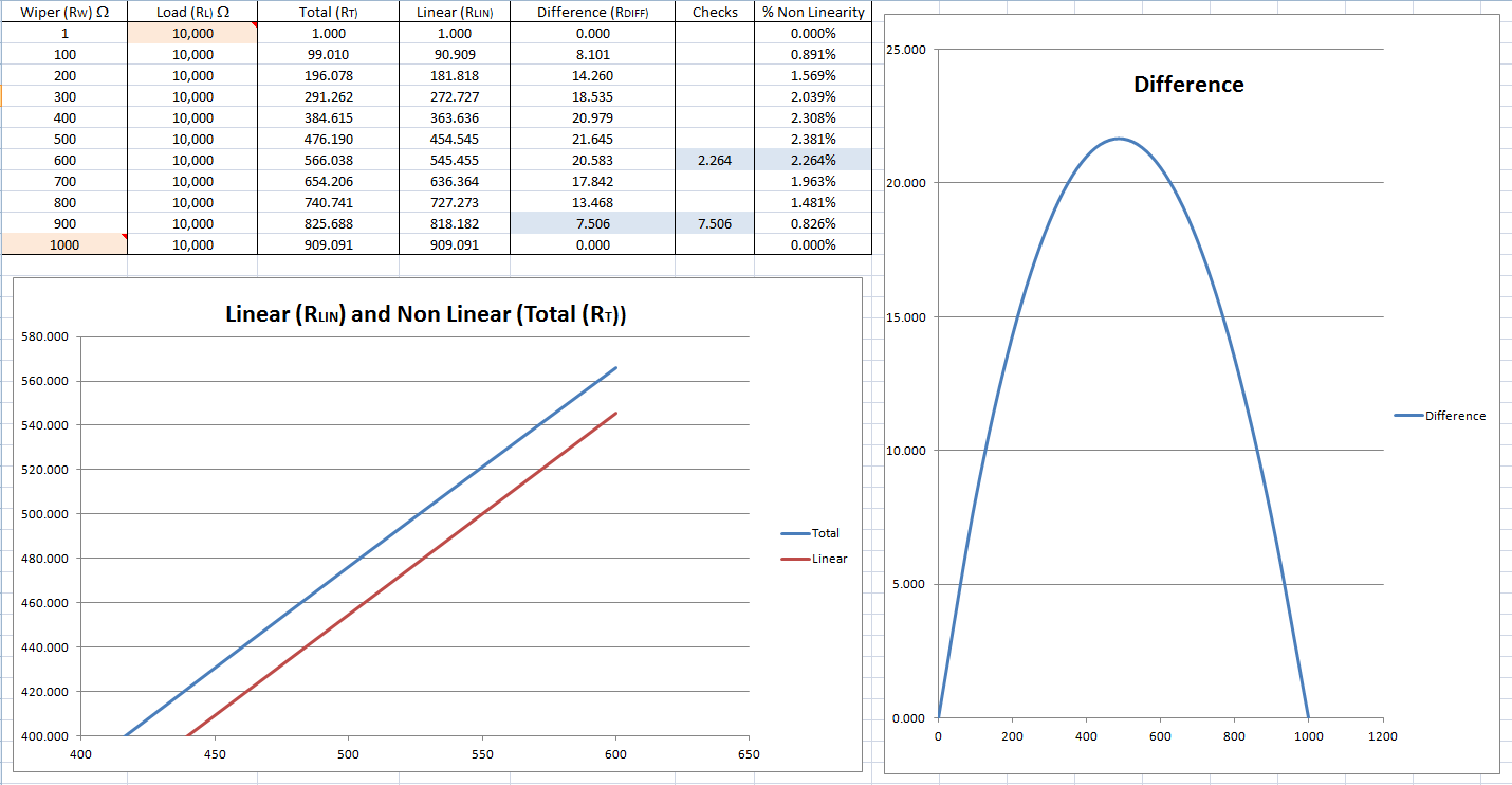
Have you ever had that terrible feeling that adding a load resistor or 'pull down' to your sensor is messing up all your analogue readings?

Maybe you're wondering why we'd want to spoil a perfectly good circuit by putting in a load resistor at all?

For many years I found that I would get strange, unpredictable, readings from my sensor related projects at the maximum and minimum locations when using analogue digital convertors (ADCs). I always blamed this on poorly designed micro processors and never for once thought that it might be my own circuit designs at fault ..... until now.

To use an analogy, when the sensor goes to maximum or minimum, it does not just reach a maximum point, but quite often actually falls off the edge of the world into a kind of no man's land where it is then prey to all kinds of digital noise and other generally nasty things like Goblins and Elves. Anybody who, like me, who has blamed this on their arduino is totally forgiven!

The example I'm using here is a simple three legged potentiometer with a ground, 5 volt and 'wiper' connection.

Using the correct pull down resistor we can eliminate noisy readings from our projects ....... And ....... just to prove that math can actually be fun .......... I'll tell you how I discovered the non linearity adjustment formula through diagrams and images.

In the circuit above we have are reading a simple potentiometer through it's 'wiper' arm through a 8.25K resistor and 16 bit ADC chip. Crucially, there is also a 100nF capacitor and a 100K resistor going to the ground rail from the wiper. We're going to concentrate on the 100K resistor. 100K is the recommended value from the manufacturers of the instrument.

There's nothing unusual about this circuit and it looks pretty boring until we look at what's happening with the resistor in more detail.

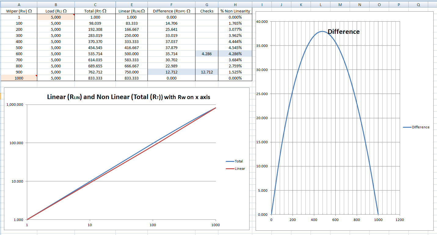
To get rid of the noises (and the Goblins and Elves) we want the resistor to be fairly small in ohms - maybe 10K, but if our pot is, for example 1K, we're going to get a massive amount of non linearity - see for yourself by opening the excel sheet in the files section.

Initially, I did not set out to discover any formulae - I just wanted to visualise the non linearity created by a load resistor in a sensor related circuit. I wanted to try and isolate the curve and plot it as a graph in Microsoft excel. It just seemed like fun.

The Math

:

I was actually working at the time on this Analogue Wind Vane project, which is basically a continuous potentiometer with a small 'dead zone' at north. Initially, the project was plagued with those familiar noisy readings until I looked at the resistor more closely.

Firstly, I plotted the actual resistance curve in Microsoft excel, which is the total resistance created by the combination of the wind vane and the load ... and I called it 'Total (RT)'. Initially, I was disappointed as I could not actually see any curve at all, so then I changed both the axes to log10. Hey presto! I can see a curve! (The blue curve on the left in the diagram above).

The total resistance is given by this well known formula:

RT w * R L ) / (Rw + RL)

• where:
• RT is the total resistance
• RW is the wiper resistance
• RL is the load resistance

OK, so far so good - not too complicated?

Next, I wanted to see how my new fancy curve looked side by side with a boring straight linear curve, just as if the results were not actually a curve at all, but a straight line. The formula for this is:

RLINw * RTMAX)/ RWMAX

• where:
• RLIN is the hypothetical linear resistance (the 'imaginary' resistance)
• RW is the wiper resistance
• RTMAX is the maximum value of the total resistance
• RWMAX is the maximum value of the wiper resistance

This is all well and good, but where are we going to get the value of the total resistance from? I really thought this was going to be easier than this, but then realised that we've already calculated this value above, it's just the maximum value of RT . But just for clarification, here is the formula:

RTMAX WMAX * R L ) / (RWMAX + RL)

• so, now, if we substitute out RTMAX we get:

RLINW * RTMAX) / RWMAX = (RW / RWMAX) * (RWMAX * RL) / (RWMAX + RL) = (RW * RL) / (RWMAX + RL)

Now we can plot our linear 'curve' (in red) and see if it's noticeably different from the curvy curve ..... and yes .... as long as we cheat by using log10, we can see the difference. If we open up the excel file, we can change the value of the load resistor to something stupidly small and get some pretty crazy curves produced.

Finally, I realised that we could then subtract the non linear curve from the linear curve and get a final outcome: the actual non linearity, or the 'difference' between the linear and non linear results. This is the pretty blue curve on the right and is given by:

RDIFFT - RLIN = (RW * RL) / (RW + RL) - (RW * RL) / (RWMAX + RL)

This equation could be reduced further, but the arduino nano is already going to struggle with some of the big numbers produced (we're working with 16 bit ADCs), so we need to help it along a little bit.

Eventually, the formula gets translated into arduino code:

////////////////////////////////////////////////////////////////////////////////////////////////////////
  // Non linearity calculations:

 load2 = load / 1000 * maxSensorValue;

  Serial.print("load2 = ");
  Serial.println(load2);

long  loadz = load2/5;
long  sensorValuez = sensorValue/5;
long  maxSensorValuez = maxSensorValue/5;

long  a = 5*((sensorValuez * loadz) / (sensorValuez + loadz));
long  b = 5*((sensorValuez * loadz) / (maxSensorValuez + loadz));

  Serial.print("a = ");
  Serial.println(a);
  Serial.print("b = ");
  Serial.println(b);
 outputValue = sensorValue + (a - b);
//////////////////////////////////////////////////////////////////////////////////////////////////////   

You'll see that the code is more 'clunky' than the formula and I've had to divide by 5 to reduce the size of some of the numbers. But it works!

Hopefully, I've now also proved not only that maths can be fun but also relevant to the real world? But what did all this work actually achieve?

If we remember from earlier on, the recommended minimum load resistor was 100K, but if we reduce these ohms we can make the readings significantly more stable near the dead zone. I tried lots of different permutations and, using the above formula to negate the non linearity, I ended up using a super accurate (+-0.1%) 30K resistor and still got good readings at due south, which, according to our excel diagram, is where most nonlinearity will occur.

Please see the 'Files' section for the excel spreadsheet.