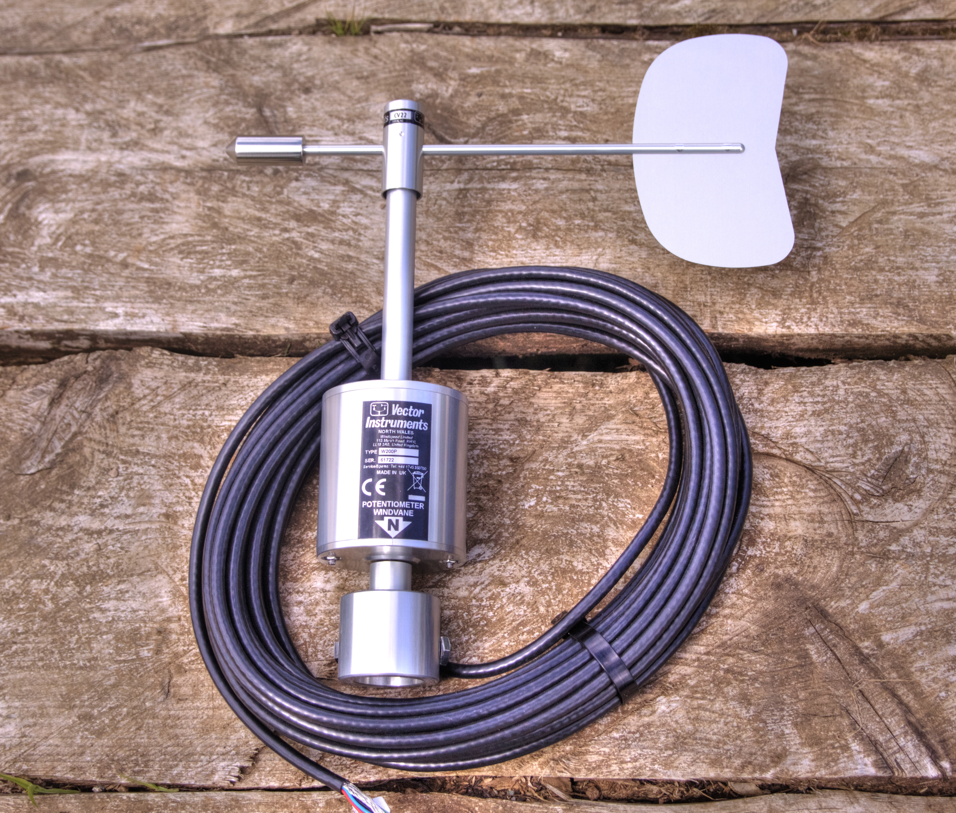
As the amazing online GPRS Weather Station project continues, we have yet another upgrade to the vast array of sensors with a professional analogue wind vane, kindly donated by Vector Instruments. This device will eventually be hooked into the new, upgraded, weather station module that I am designing. The current prototype is producing live data here: http://www.goatindustries.co.uk/weather2/ .

Comparing this sensor to my DIY Digital Wind Vane the first thing I noticed was the extreme sensitivity to wind movement - it has very low torque - so it is able to pick up wind direction even in very small wind speeds. Secondly, being made on a CNC lathe, the quality of the engineering is superb - I really must get myself a CNC lathe!

Here, I am going to show how I set up and coded an arduino to read the sensor, made calculations for non-linearity, took account of the 'dead zone' in the potentiometer, turned the readings into a large numerical array, efficiently calculated the mode value and made the whole device set itself up automatically. No pressure!

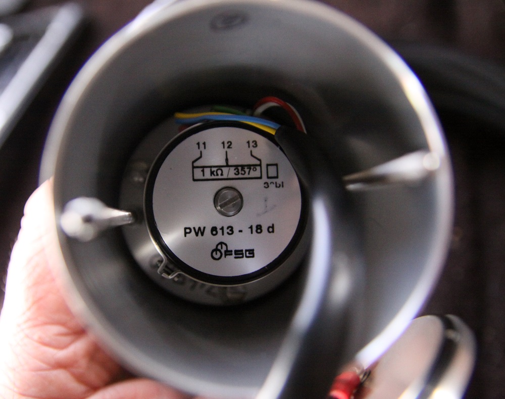
This analogue wind vane is based on a very expensive potentiometer with three main connections - 5V, ground and wiper. The wiring inside the deice is very thin so great care is needed not to put too much current through the circuits for too long or it could quite easily get burnt out.

I have protected the wiper part of the circuit with a 10k resistor which feeds a signal to the arduino via pin A0. This is then converted into a digital 10 bit code inside the processor with a full range of 0 to 1024. The device is never fed a continuous supply of power and is pulsed in two different ways. Firstly, there is a load of really fast 50 millisecond pulses which gets us 10 readings at a time, next the whole device goes off for 1/2 a second until the next batch of readings is made. By working out an average (mean), we end up with one fairly accurate reading per second.

So now that we've got this digital reading - what else could be simpler? Surely that's the end of it?

Firstly, when working with analogue to digital conversion in the past, I have noticed significant 'drift' around minimum and maximum values and so some code is going to need to be written to counteract this phenomenon. Secondly, wind can sometimes be extremely turbulent which makes it very difficult to get an accurate output value. If the wind was constantly changing from, say, south to west we would want to process our data in such a way that it would give the most common direction, not just the average or 'mean', otherwise we would just get a value of south-west. To explain in more detail - the wind might veer from south to west and back again, but actually it's mostly coming from the south-south-west. If this is beginning to hurt your brain cells, I totally sympathise!

Fortunately we have solutions to both the above problems - we take as many readings as the system memory and speed will allow and build some truly massive arrays of numbers. We then make a continuous log of the number of times each part of the array is hit and then, finally, spit out the most popular. In the digital wind vane project I wrote some rather clunky code for calculating the 'mode' value and now, with the power of some extra nutritious coffee granules, I have reduced that code to something rather more sublime!

Finally, after about ten minutes, just when our arrays are about to explode the arduino into a million fragments of silicon dust, we retrieve a single wind direction value eg 215 with a second arduino and reset all the large numbers to zero.

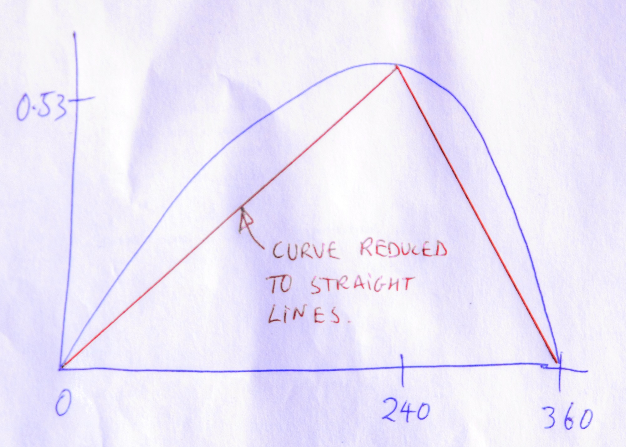
Now that we're beginning to feel quite glib about our engineering prowess, the analogue wind vane chucks at us 2 more major problems - ONE: With the recommended 100K load in place, it does not produce a true linear output and TWO: it has a dead zone around the north pole of about 3 degrees. At first, my brain cells started to panic at the prospects of solving the non linearity problem but then they remembered that wind is always slightly turbulent so the question arose: How accurate do we really need to be? Do we really need to look into a lot of detail at the non linearity curve? Common sense then came to the rescue and the curve got chopped and straightened into 2 simple straight lines, with an apex at 240 degrees. Simple!

Parts:

1. C1 Ceramic Capacitor voltage 6.3V; capacitance 100nF
2. J1 Piezo Speaker
3. LED1 Green (560nm) LED package 5 mm [THT]; leg yes; color Green (560nm)
4. Part1 Arduino Nano (Rev3.0) type Arduino Nano (3.0)
5. R1 100 Resistor resistance 100; package THT; bands 4; tolerance ±5%; pin spacing 400 mil
6. R2 2k Resistor resistance 2k; package THT; bands 4; tolerance ±5%; pin spacing 400 mil
7. R3 8.25k Resistor resistance 8.25k; package THT; bands 4; tolerance ±5%; pin spacing 400 mil
8. R5 100k Resistor resistance 100k; package THT; bands 4; tolerance ±5%; pin spacing 400 mil
9. S1 Pushbutton package [THT]
10. W200P wind vane from Vector Instruments
11. ADS1115 ADC

Arduino Setup

:

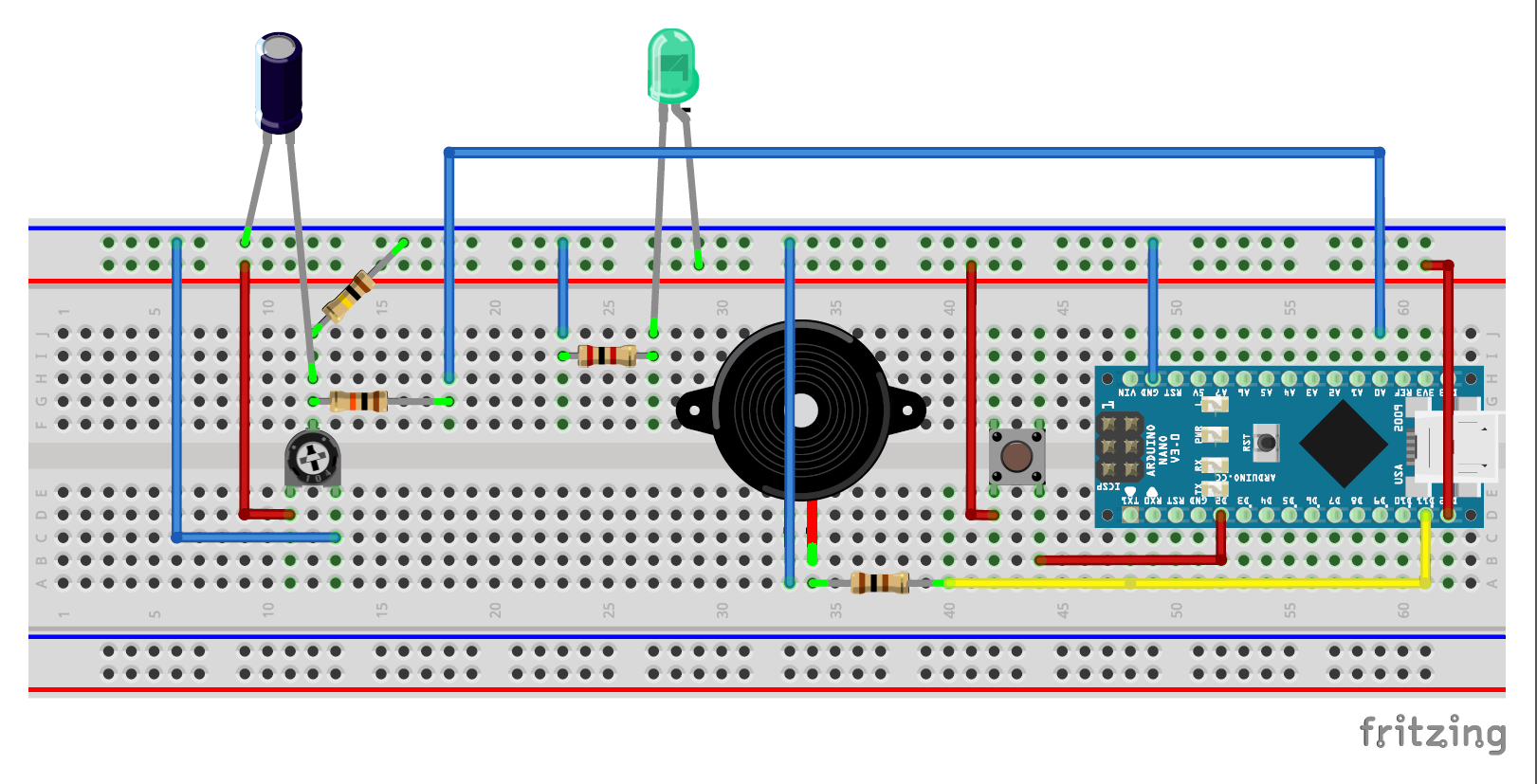
This is the easy and fun part and we can make lots of reassuring beeping noises and flickering of LEDs to make us feel better after having brutalised our brain cells so much in the previous steps. The LED flickers because the power supply is being pulsed and the micro speaker beeps when we have got the wind vane in the self calibration zone.

After wiring up the breadboard, we connect the power and point the wind vane to due north, which will be in the dead zone. We then move the vane very slightly to the left and right and there should be beeping noises produced in two separate audio frequencies, representing minimum and maximum range settings being discovered. Do this a couple of times and the sensor is set up and ready for use until the power is disconnected again.

As time goes on, but only when the wind is blowing roughly from the north, the maximum calibration setting is very slowly decreased, or pulled back, until it is over-ridden by a new setting. The same happens with the minimum setting, but in the opposite direction, i.e. pushed forwards.

I did also play about with the capacitor on the wiper pin and found that a 100 nano farad capacitor worked better than the 10 nano farad proscribed in the data sheets in terms of the stability of the end point values. This will, however, affect the sensitivity of the device as it sweeps backwards and forwards over the dead band.

const int analogInPin = A0;  // Analog input pin that the potentiometer is attached to
const int analogOutPin = 9; // Analog output pin that the LED is attached to
const int tonePin = 11; 
int sensorValue = 1;          
float outputValue = 0;
float rawDirection =0;
float maxSensorValue =980.9999;
float minSensorValue = 5.0001;
int finalDirection=0;
int biggestAddingDirection=0;
int z=0;
int sensorValue2=0;
int n=0;
int modeSize=0;
int c=0;
int degree =0;
int addingDirection[]=
  {1,2,3,4,5,6,7,8,9,10,11,12,13,14,15,16,17,18,19,20,21,22,23,24,25,26,27,28,29,30,31,32,33,34,35,36,37,38,39,
  40,41,42,43,44,45,46,47,48,49,50,51,52,53,54,55,56,57,58,59,60,61,62,63,64,65,66,67,68,69,70,71,72,73,74,75,76,77,78,79,
  80,81,82,83,84,85,86,87,88,89,90,91,92,93,94,95,96,97,98,99,100,101,102,103,104,105,106,107,108,109,110,111,112,113,114,115,116,117,118,119,
  120,121,122,123,124,125,126,127,128,129,130,131,132,133,134,135,136,137,138,139,140,141,142,143,144,145,146,147,148,149,150,151,152,153,154,155,156,157,158,159,
  160,161,162,163,164,165,166,167,168,169,170,171,172,173,174,175,176,177,178,179,180,181,182,183,184,185,186,187,188,189,190,191,192,193,194,195,196,197,198,199,
  200,201,202,203,204,205,206,207,208,209,210,211,212,213,214,215,216,217,218,219,220,221,222,223,224,225,226,227,228,229,230,231,232,233,234,235,236,237,238,239,
  240,241,242,243,244,245,246,247,248,249,250,251,252,253,254,255,256,257,258,259,260,261,262,263,264,265,266,267,268,269,270,271,272,273,274,275,276,277,278,279,
  280,281,282,283,284,285,286,287,288,289,290,291,292,293,294,295,296,297,298,299,300,301,302,303,304,305,306,307,308,309,310,311,312,313,314,315,316,317,318,319,
  320,321,322,323,324,325,326,327,328,329,330,331,332,333,334,335,336,337,338,339,340,341,342,343,344,345,346,347,348,349,350,351,352,353,354,355,356,357,358,359,360,361,362};
  
void setup()
{
  pinMode (12,OUTPUT);         // This provides short pulses of power to the sensor from pin 12.
  pinMode (13,OUTPUT); 
  pinMode(2, INPUT_PULLUP);
  digitalWrite(13, LOW); 
  Serial.begin(9600);
  while (degree<362)           // Set all 362 values to zero.
  {
    addingDirection[degree] = 0;
    degree++;
  }
  maxSensorValue =984.9999;
}

void loop() 
{
  resetValues();
  z=0;
  n++;
  sensorValue2=0;
  
  while (z<10)                             // Get 10 quick readings.
    {
    z++;  
    digitalWrite(12, HIGH);
    delay(5);
    // read the analog in value:
    sensorValue = analogRead(analogInPin);
    sensorValue2 = sensorValue2 + sensorValue;
    digitalWrite(12, LOW);
    delay(45);
    }
  
  delay(500);                            // set this to 500 so total delay = 1 second.
  sensorValue = (sensorValue2/z);
  // assume that dead band starts at 356.5 and ends at 0
  // and values of zero correspond to 360 or 0 degrees:
  // The maximum analogue reading I am getting on the wiper is 981
  // out of a possible range of 1024 (10 bits)
  
  if (sensorValue == 0)
  {
    outputValue =0;
  }
  
  outputValue = ((sensorValue-minSensorValue)*356.5/maxSensorValue)+1.75;
  
  selfCalibrate();                         // Checks the maximum range of the analoue readings when sensor comes out of dead band.

////////////////////////////////////////////////////////////////////////////////////////////////////////
  // Non linearity calculations:
  // Now assume that max non linearity is at 240 degrees and is +0.53
  // Also, assume non linearity itself is linear, not a curve:

  if (outputValue<240 || outputValue==240)
  {
    rawDirection = outputValue*0.53/240 + outputValue;
  }
  if (outputValue>240)
  {
    rawDirection = 0.53*(358-outputValue)/118 + outputValue;
  }
  if (sensorValue == minSensorValue) 
  {
  rawDirection=360;
  }
////////////////////////////////////////////////////////////////////////////////////////////////////// 
  Serial.print("sensor = ");
  Serial.print(sensorValue);
  Serial.print("\t output = ");
  Serial.print(outputValue,2);
  Serial.print("\t adjusted output = ");
  Serial.print(rawDirection,2);
  Serial.print("\t Max sensor value = ");
  Serial.print(maxSensorValue,2);
  Serial.print("\t Min sensor value = ");
  Serial.print(minSensorValue,2);
  Serial.print("\t n = ");
  Serial.println(n);  

  digitalWrite(12, LOW);

 degree = (int)rawDirection;

/////////////////////////////////////////////////////////////////////////////////// 
 // Special case for rawDirection = 360:
 if (rawDirection ==360)
 {
  degree = 359 + c;
  c++;
 }
 if (c>2)
 {
  c=0;
 }
 if (degree==361)
 {
  degree=1;
 }
/////////////////////////////////////////////////////////////////////////////////////  
// Calculate the running mode (Some of these variables will need to be reset by a call back from main processor).

 addingDirection[degree] = addingDirection[degree] +1;
if (addingDirection[degree] > modeSize)
{
  modeSize = modeSize +1;
  finalDirection = degree;
}

//////////////////////////////////////////////////////////////////////////////////////
if (finalDirection==359 || finalDirection==360 || finalDirection==1)
{
  finalDirection=360;
}
  Serial.print("Mode size = ");
  Serial.print(modeSize);
  Serial.print("\t Degree = ");
  Serial.print(degree);
  Serial.print("\t Final Mode Direction = ");
  Serial.print(finalDirection);
  Serial.print("\t Adding direction[degree] = ");
  Serial.println(addingDirection[degree]);

  Serial.println(""); 

}
// 30 days = 2592000 seconds
// Each loop of n x 10 is ten seconds
// Every ten seconds max sensor value is reduced by 0.0001
// Every 30 days max sensor values reduced by 2592000 / 10 * 0.00001 = 25.92 degrees
// In 3 days of northerly winds max sensor value will adjust by as much as 2.592 degrees.
// During northerly winds the sensor will self calibrate:

void selfCalibrate()
{
if (sensorValue > maxSensorValue)
  {
   maxSensorValue = sensorValue;
   tone(11,1000,500);
  }
if (sensorValue < minSensorValue)
  {
   minSensorValue = sensorValue;
   tone(11,2000,500);
  }
  
if (  ((n>10)&&(sensorValue>900)) || ((n>10)&&(sensorValue<100))   )            // Only adjust min and max sensor readings in a northerly wind.
  {
  maxSensorValue = maxSensorValue - 0.01;                                       // Slowly pulls back max sensor value.
  minSensorValue = minSensorValue + 0.01;                                       // Slowly pushes forwards min sensor value.
  n=0;  
  }
}
void resetValues()                                        // Requires a call back pulse of 5 seconds to reset key values.
{
  int callBack = digitalRead(2);
  if (callBack==LOW)
  {
    digitalWrite(13, HIGH);
    modeSize=0;
    tone(11,2500,500);
    while (degree<362)
    {
    addingDirection[degree] = 0;
    degree++;
    }
  }
  else
  {
  digitalWrite(13, LOW); 
  }
}

// This bit of code below takes care of the instance where the weather vane is hovering around north (hovering zone) and picking up big values and small values in the same batch of 11:
// Total range is about 0 to 24000.
//////////////////////////////////////////////////////////////////////////////////////////////////////////////////////////////////////                                                              
     if (adc0 < 12000)
      {
       sensorValue4 = sensorValue4 + adc0;
       small++;
      }
     if (adc0 >= 12000)                                    
      {
       sensorValue3 = sensorValue3 + adc0;
       big++;                                          
      }
     if (big > small)
      {
       sensorValue = sensorValue3 / big;     
      }
     if (big < small)
      {
       sensorValue = sensorValue4 / small;
      }
///////////////////////////////////////////////////////////////////////////////////////////////////////////////////////////////////////

void variation()
{
  maxValue = max(sensorValue,maxValue);
  minValue = min(sensorValue,minValue);
  variability = maxValue - minValue;
  Serial.print("Variability in the reading = ");
  Serial.println(variability);
}

////////////////////////////////////////////////////////////////////////////////////////////////////////
  // Non linearity calculations:

 load2 = load / 1000 * maxSensorValue;

  Serial.print("load2 = ");
  Serial.println(load2);

long  loadz = load2/5;
long  sensorValuez = sensorValue/5;
long  maxSensorValuez = maxSensorValue/5;

long  a = 5*((sensorValuez * loadz) / (sensorValuez + loadz));
long  b = 5*((sensorValuez * loadz) / (maxSensorValuez + loadz));

  Serial.print("a = ");
  Serial.println(a);
  Serial.print("b = ");
  Serial.println(b);
 outputValue = sensorValue + (a - b);
//////////////////////////////////////////////////////////////////////////////////////////////////////