I am a final year Mechatronic Engineering student at the University of Manchester. For details about me please click here.
The potential use of this product is demonstrated by the following video where the camera tracks the motion, orbits around the point of interest and rotates about itself, creating an extraordinary footage.
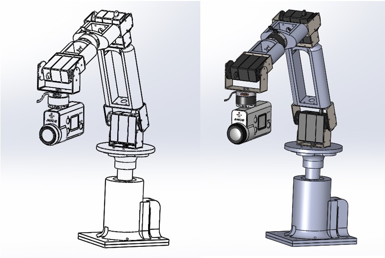
The simulation of the product is as follows:
Note that the blue arrow shows the direction at which the camera is pointing. Also, the trajectory that is given in red, can be altered as desired using the Virtual Reality add-on.
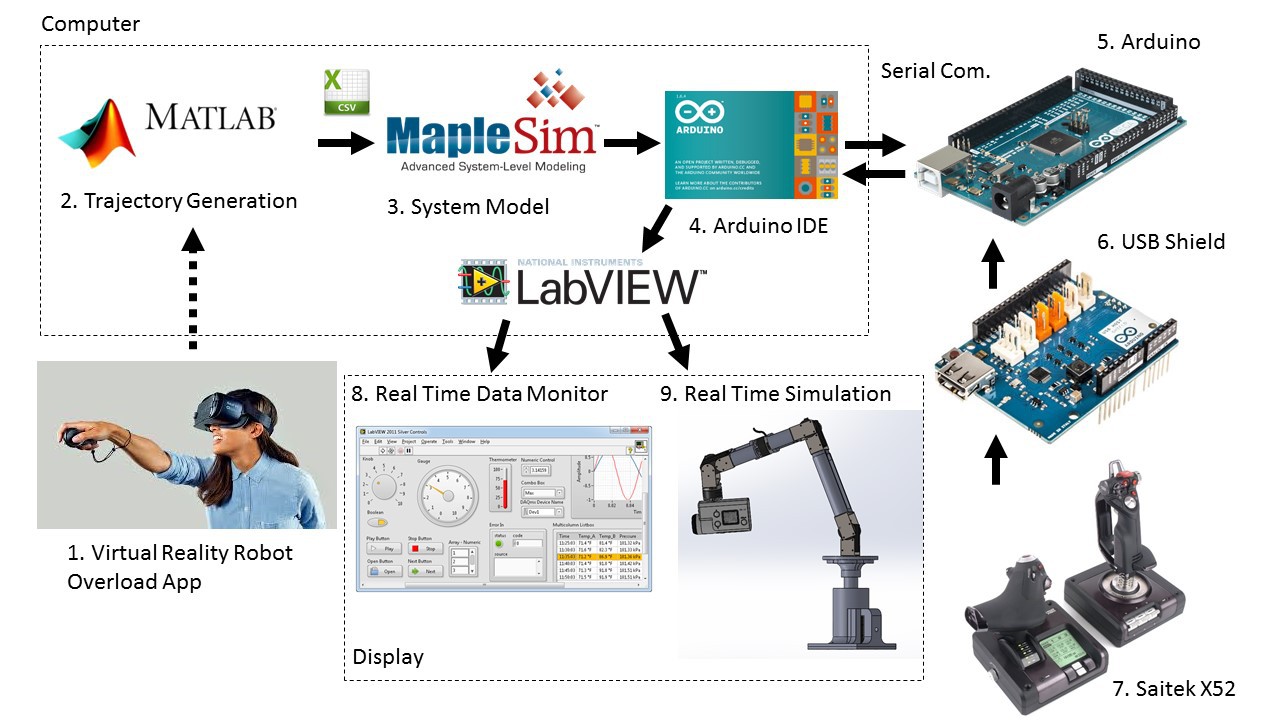
- Virtual Reality is an optional step for producing the intermediate positions in the camera trajectory.
- Trajectory generation: Given start, end, and intermediate positions, the quantic trajectory polynomial generates the end-effector trajectory in MATLAB.
- These Cartesian coordinates are exported to the robot manipulator simulation.
- If the simulation works as expected, the trajectory is transmitted to the microcontroller via serial communication.
- The camera orientation can be controlled by a human operator or by the object detection algorithm.
- The position feedback is transferred into the LabVIEW environment and used for monitoring the data and simulating the results on the 3D model.
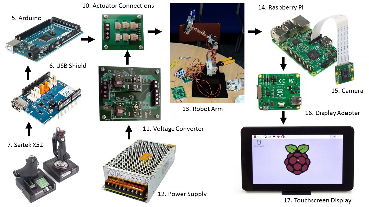
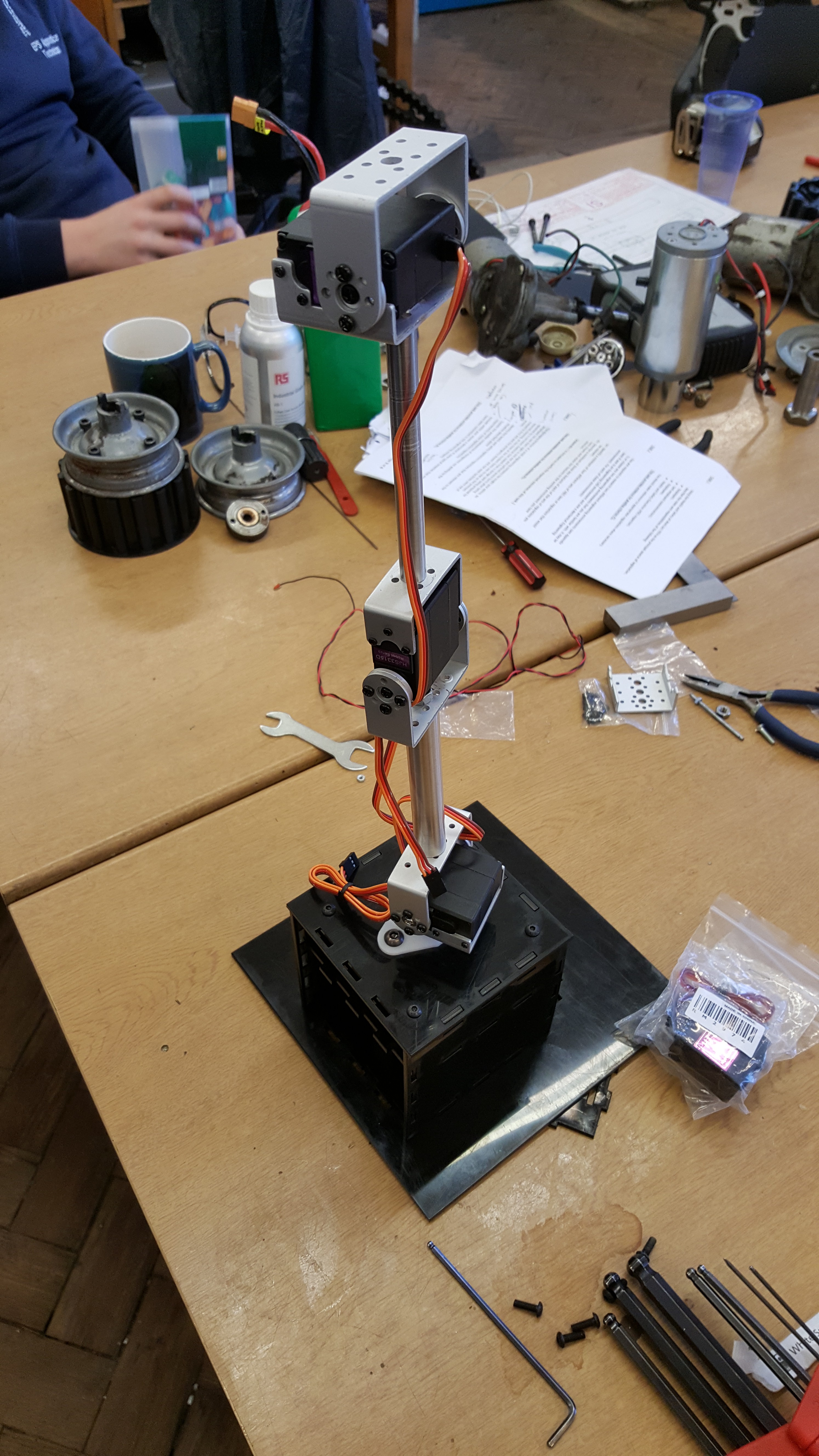
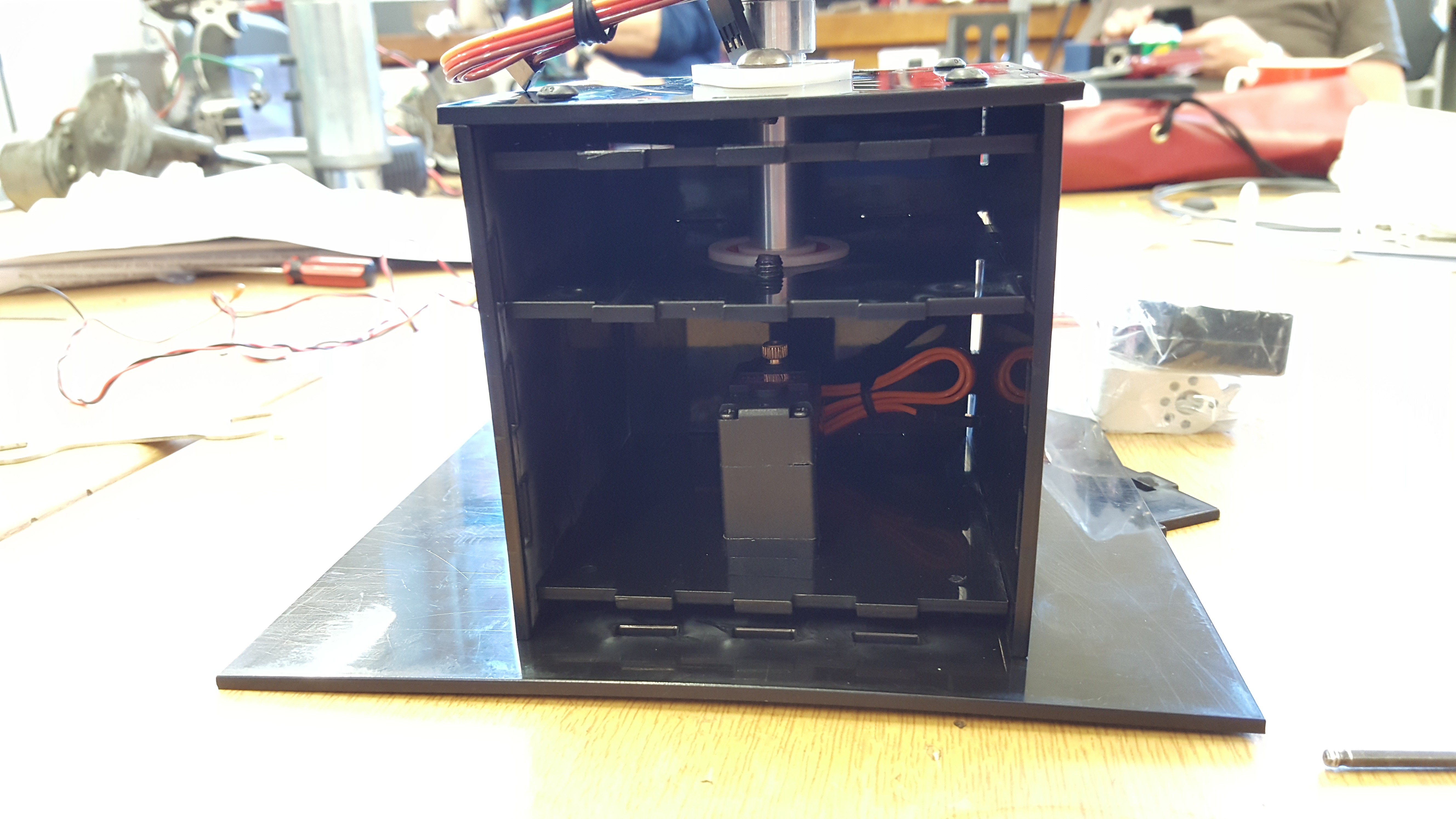
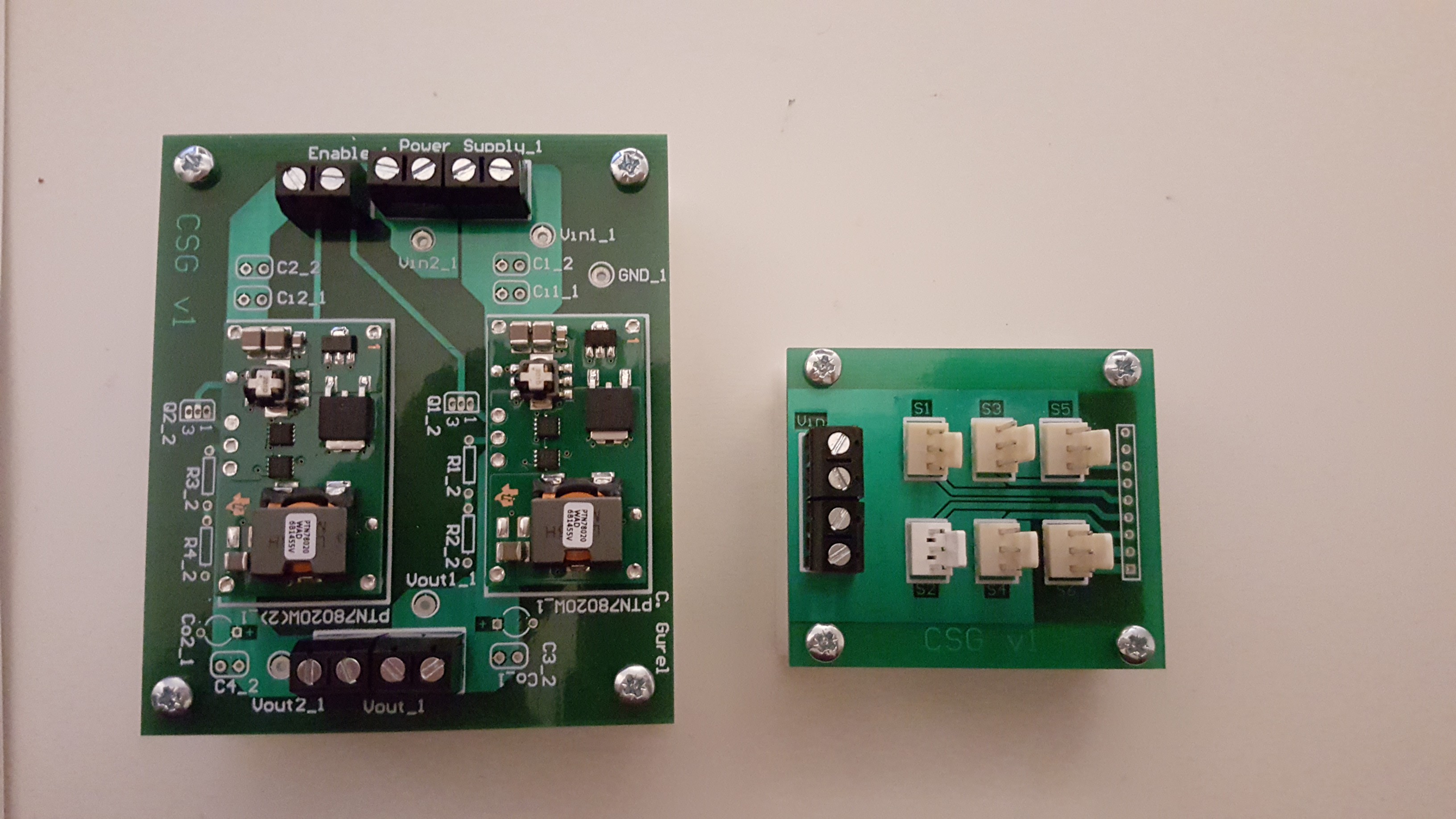
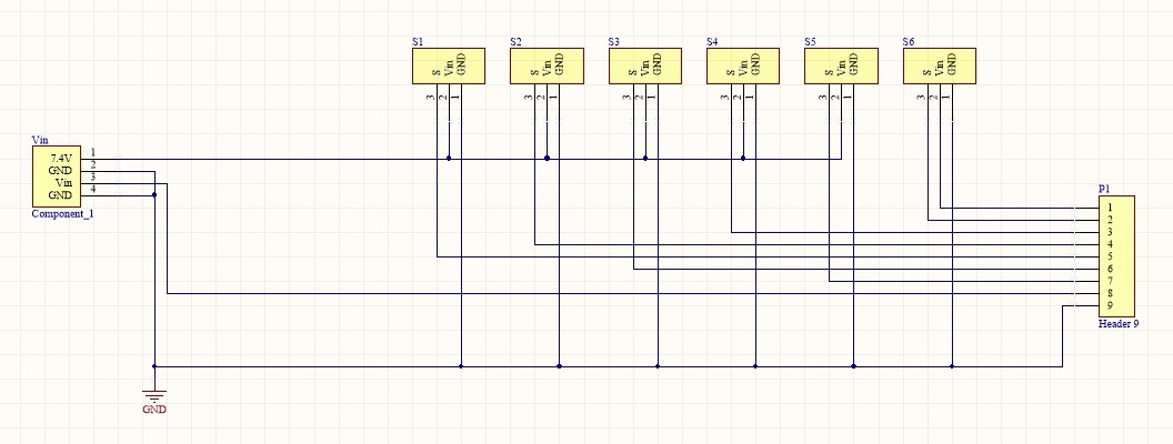
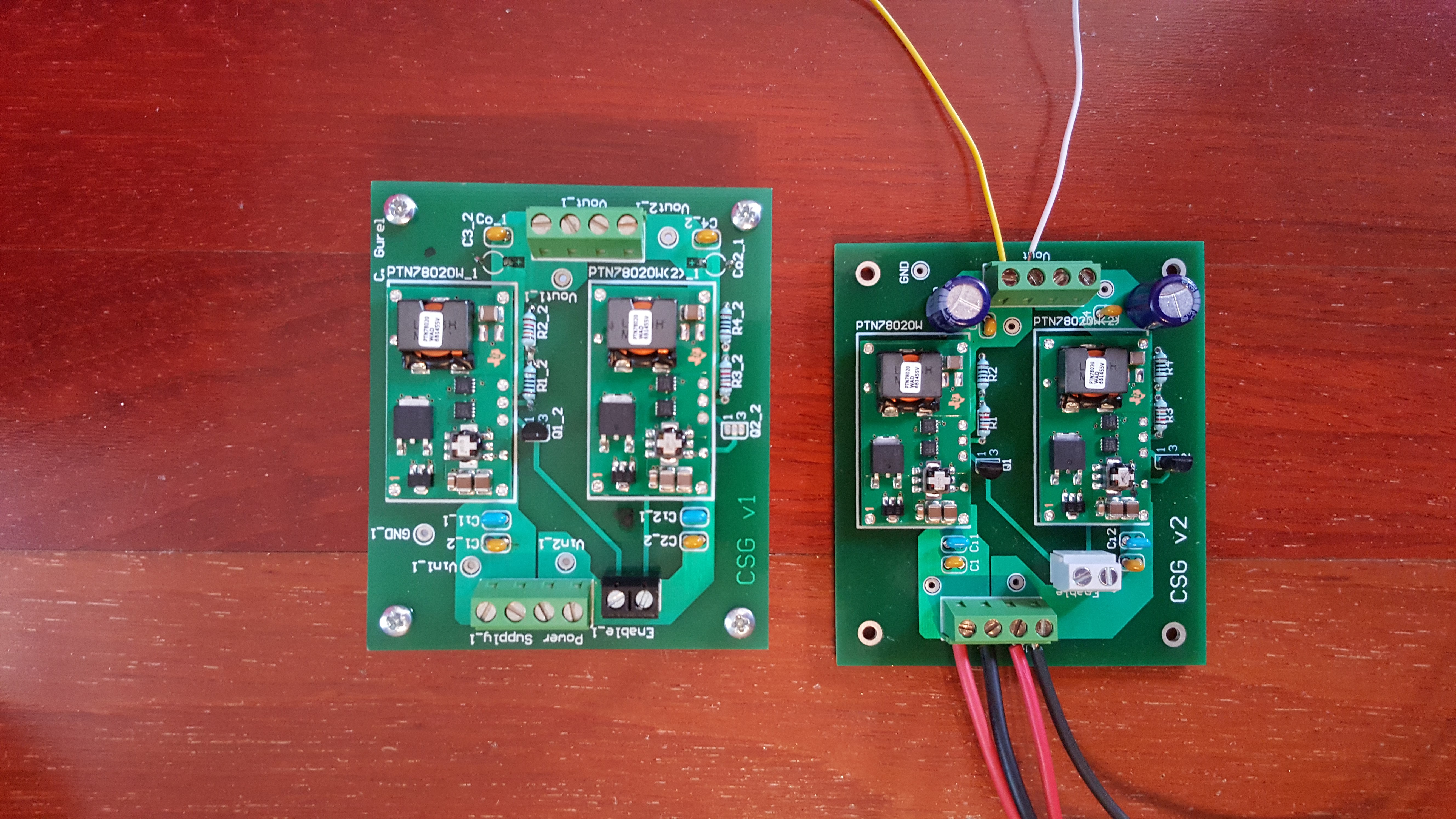
The circuitry is completed. An image is provided below.
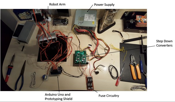
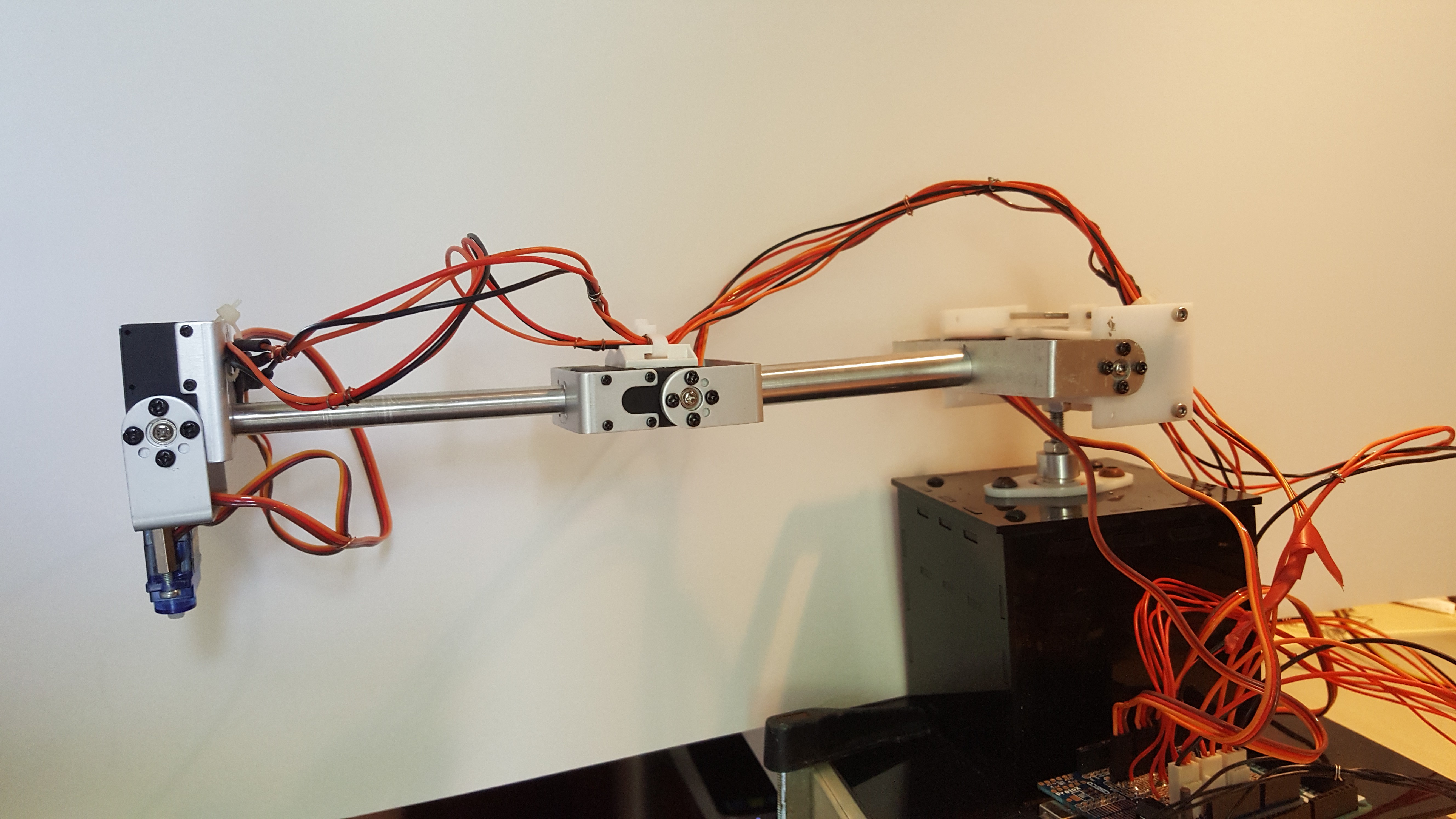
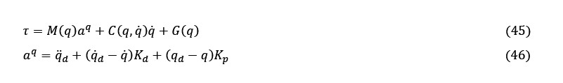
 Figure 4.30 demonstrates the inner loop and outer loop control architecture where the output of the system yields the joint space signal which enables a better trajectory tracking given that the feedback gains and are tuned as appropriate.
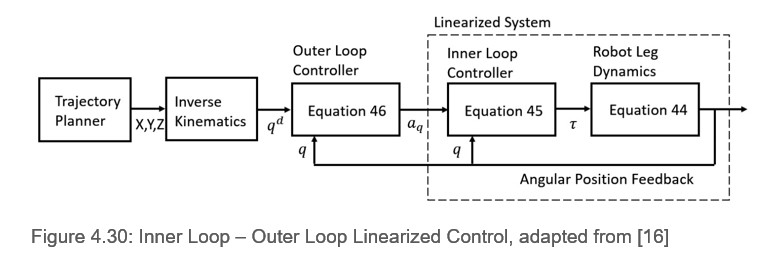


 Petar Crnjak
 Piotr Sokólski