Like any sensor information, there will always be some inherent noise associated with the output data. This is practically unavoidable as anything that has free flowing electrons will have an associated thermal noise with it, among other sources. This is the main reason why you get grainy images on a digital camera at low light values.

So how do we deal with it. The first and easiest method is to just ignore it and move on. However, these higher frequency effects can play havoc with some control system. If you look at the MappyDot's raw data output from some still, medium and fast motion (measurement rate of 30Hz), you will see many higher frequency "spikes" on the data, which if used on robotics, can be translated into large acceleration values if you don't account for it on a smaller timescale (by filtering):

To help with this, each MappyDot will by default actually do some of this filtering for you which reduces the processing overhead required to filter data from numerous sensors at once for general and rapid motion cases. You can turn this filtering off on the MappyDot if you want higher frequency motion data.

To do this, we first needed to design a filter that would be both useful and not lose too much information. We want something that can limit any higher frequency effects as they arrive into the system. Limit here being the key term, as it will smooth incoming data and still maintain "lower" frequency response.

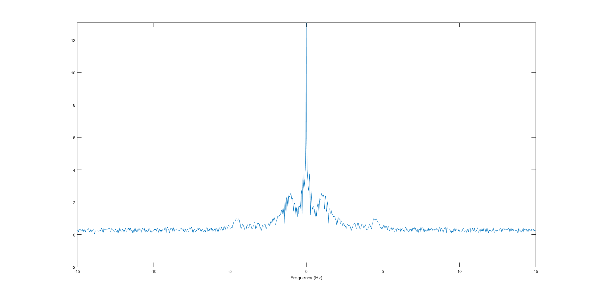
If we look at the FFT of the dataset, we can see that after 5-6Hz, there is no significant changes apart from noise:

Using Matlab, we can create a simple low pass filter to help cut off these values and to analyse the changes made by changing certain coefficients. This won't be the final design of the filter implementation as it needs to work realtime, however we can play around with this to optimise the cutoff frequency for decent looking results.

filename = '..\filtering_raw_data';
A = importdata(filename);
clf
hold on
plot(A)
fNorm = 3 / (30/2); %3Hz cutoff frequency, 30Hz sample rate
[b, a] = butter(10, fNorm, 'low'); %Butterworth filter with order 10
Y = filtfilt(b, a, A);
plot(Y);

Note that filtfilt "performs zero-phase digital filtering by processing the input data, x, in both the forward and reverse directions". So the actual implementation will have a small delay depending on the order value since we don't know the complete waveform as it comes in. This delay however can be exceptionally small (~<33ms), so it shouldn't affect the output so much if the filter is turned on. And since this is performed on the MappyDot, if you are reading this data at a slower rate (<30Hz) with another device, this delay will not be noticed. Some more reading here and here.

0.3Hz cutoff (really bad fit, most information lost):

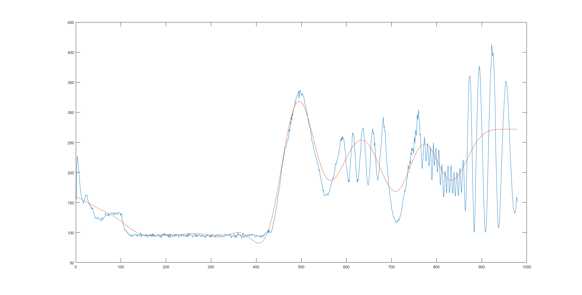
1Hz cutoff (getting better, still loss of information):

3Hz cutoff (much better fit, but fast motion is still cut off):

4Hz cutoff (similar to 3Hz):

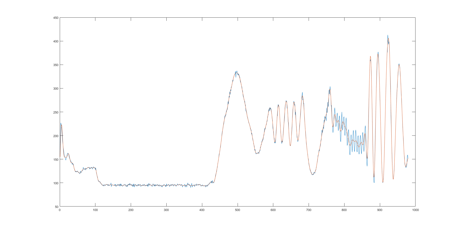
5Hz cutoff (much better fit with faster movements, although there is still some bad fitting, high frequency noise effects are cutoff):

6Hz cutoff (very good fit for faster movement, high frequency effects are still smoothed out):

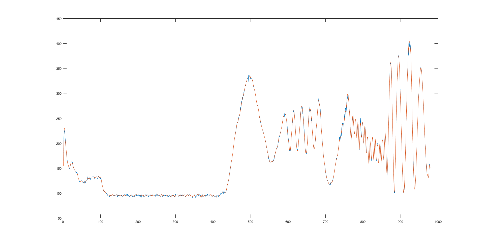
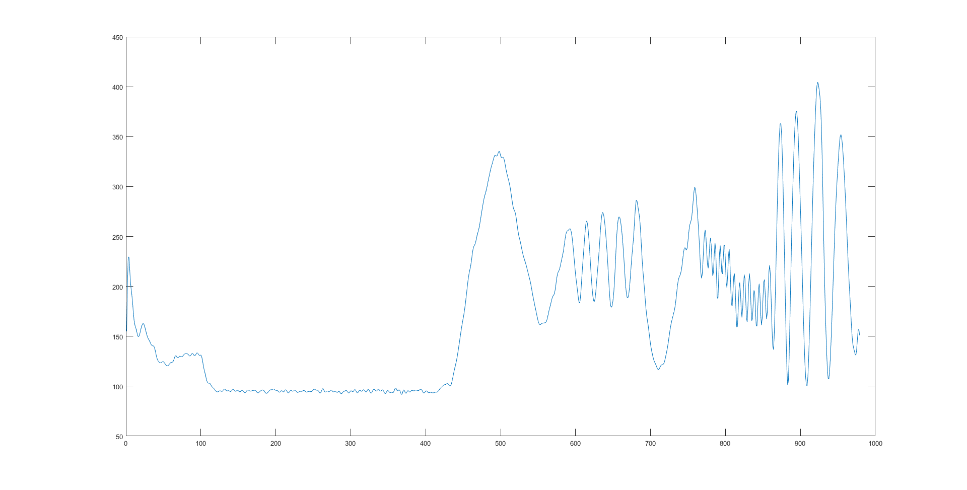
And if we look at the 6Hz cutoff by itself:

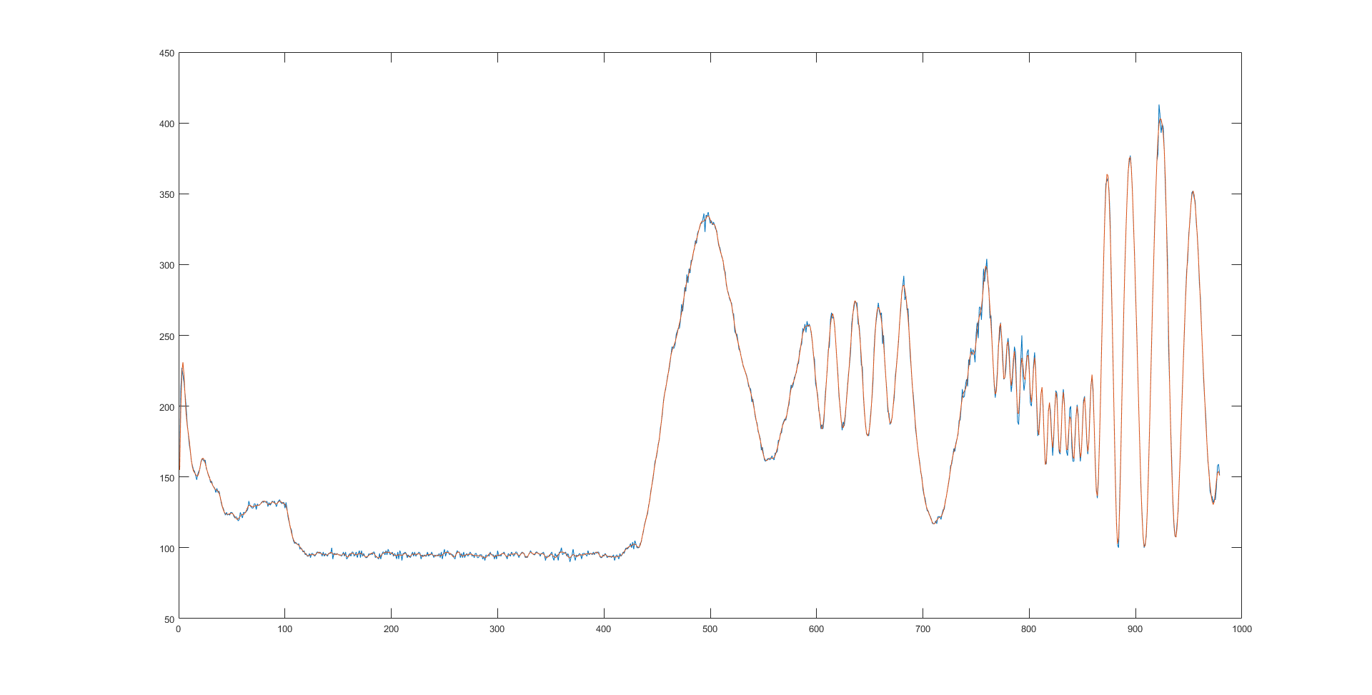
If you compare that to the original data above, you will see that you get a pretty good representation of the data without too much information loss. Going much higher than 6Hz causes the data to start to fit to the higher frequency "spikes".