 Stephanie Stoll
This log goes into detail about the implementation of the high level control. For a reminder on what the system looks like on a more basic level see a previous log called Introduction to Vision-Based Learning.
Combining Caffe, OpenCV, and Arduino
A Python script combines the Caffe-trained AlexNets, the OpenCV camera feed and communication with the Arduino Mega 2560. This script is used to control the hand from the command line giving only a closing command. The open command is issued automatically but this could be easily changed to manual operation. The script demonstrates the simplicity of the hand’s interface, with most of the complex work carried out by the CNNs. You can find the script under files.
Let's look more closely at how Caffe defines CNNs and how data is processed.
CNNs in Caffe
In Caffe deep networks are defined layer-by-layer in a bottom-to-top fashion, starting at input data and ending at loss. Data flows through the network as blobs in forward and backward passes. A blob is Caffe’s unified data representation wrapper. A blob is a multi-dimensional array with synchronisation abilities to allow for processing on the CPU as well as GPUs, that can hold different kinds of data, such as image batches, or model parameters. Normally, blobs for image data are 4D, with batch-size x number-of-channels x height-of-images x width-of-images.
Blobs are processed in layers. A layer inputs through bottom connections and outputs through top connections. Below shows the definition of a convolution layer in plaintext modelling language on the right, and visualised as a directed acyclic graph (DAG) on the left:
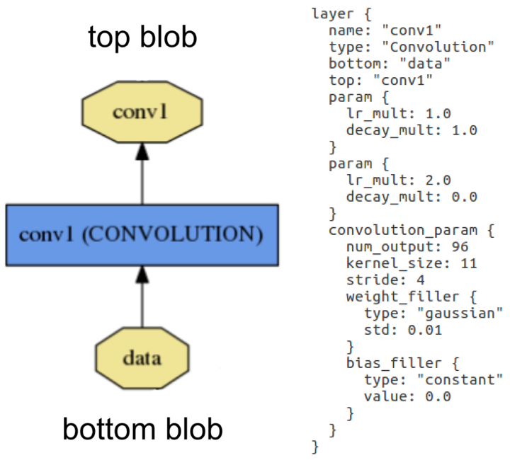 Layer example: Layer "conv1" takes in data through bottom connection and outputs conv1 through top connection. Parameters for convolution operation are defined in the net's prototxt file and can be visualised as a DAG (directed acyclic graph).
Layers are responsible for all computations, such as convolution, pooling, or normalisation. A set of layers and their connections make up a net. A net is defined in its prototxt file using a plaintext modelling language. Normally, a net begins with a data layer, that loads in the data and ends with a loss layer that computes the result (classification in our case). The weights for the net are adjusted in training and are saved in caffemodel files.
The figure below shows a DAG visualisation of Yann LeCun’s LeNet-5. In this case, the network is configured to train in batches of 64 images. Images are scaled before being put through the first convolution stage. The first convolution stage has an output of 20 per image. The outputs are pooled using max-pooling before being put through the second convolution stage with 50 outputs per image, followed by another pooling stage. Data then enters the fully connected layers, in which the first inner product layer computes the inner product between the input vector and the weights vector with an added bias, producing 500 outputs that are then rectified using a sigmoid. This output is fed into a second inner product layer which produces an automatically calculated number of outputs (or it can be defined in the prototxt file). Finally, loss and accuracy are computed by comparing the results of the second inner product (ip2) to the labels, whereas softmax reflects the likelihoods of each class computed in ip2.
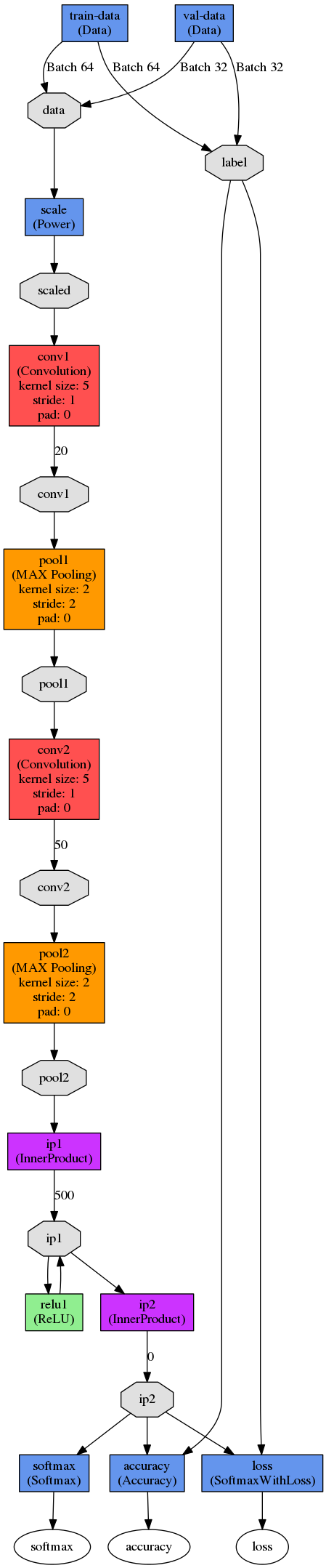
LeNet-5 was developed for character recognition and works on small 28x28 pixel images. It was only used in this project to understand the fundamental principles of deep networks. For our high-level control, we used five instances of a pre- trained AlexNet which was designed in 2012 for the ImageNet Large-Scale Visual Recognition Competition (ILSVRC).
AlexNet
The AlexNet architecture is similar to the LeNet but more complex. It has five convolutional and three fully connected layers and randomly crops 224x224 patches from an input image, meaning effectively less data is needed. AlexNet contains 650,000 neurons, 60,000,000 parameters and 630,000,000 connections. As the dataset collected for this project is too small to train a network of this size, I used pre-trained AlexNets and only re-trained the fully connected layers with test data from my collected dataset. For more information on the data used and the training process see the future log on Data Collection and Training.
Let's look at how the CNNs are trained using Caffe and Digits are used in the high-level control.
Putting CNNs to Use
In order to classify an image at runtime using the CNNs they need to be imported and set up using the pyCaffe module. To import and set up a CNN pyCaffe requires the net’s prototxt file as well as a caffemodel file. The mean of all images the net was trained on, is subtracted from any incoming image. This net, as well as all the others used in this project were pre-trained on the ImageNet dataset, hence the mean of these images is used. After initialising the net a camera feed is set up using OpenCV’s python library ‘cv2’. A transformer is then set up that is responsible for pre-processing image data into a Caffe blob compatible format to be pushed into the network. A frame is read from camera and resized to the dimensions expected by the net, before being pushed into the network by the transformer. The net returns probabilities for all classes after a forward pass.
The next log will discuss how the CNNs where trained for the system and what data was used, as well as describing the data collection and augmentation process.
Discussions
Become a Hackaday.io Member
Create an account to leave a comment. Already have an account? Log In.