 M. Bindhammer
I should have thought about the Beer-Lambert Law earlier!
where
- A: Absorbance or optical density OD of the wave length λ
- I_0: Intensity of light that is incident on the sample [W·m^(−2)]
- I_1: Intensity of light that is transmitted by the sample [W·m^(−2)]
- ε: Molar extinction coefficient of the wave length λ [L·mol^(–1)·cm^(–1)]
- c: Concentration [mol/L]
- l: Length of the light path through the sample, usually 1 cm
Spectrophotometers are commonly used to measure the concentration of a solution from its light absorbing properties. Some other examples of how they are used include:
- Water quality - Turbidity, chlorine content, pH, water hardness, phosphate content etc
- Microbial population growth - Turbidity of a microbial culture over time
- Enzyme kinetics - Activity of an enzyme over time
For RGB spectrophotometry we can use a RGB LED and the TCS3200 color sensor, which output is a square wave (50% duty cycle) with frequency directly proportional to light intensity.
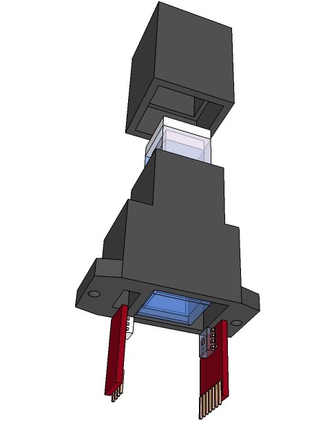
Proposed design, directly mountable on a PCB (complete copper fill without traces on both layers of the board in the area of the cuvette bottom to avoid exposure to light through the PCB):
As initially mentioned one use of the spectrophotometer is to determinate microbial population growth. How we do that? Let's start with a exponential bacteria growth model. Let donate the increase in cells numbers ΔN per time interval Δt, then this ratio is proportional to the actual number of cells N. If for example a population of 10000 cells produces 1000 new cells per hour, a 3 times bigger population of the same microorganism will produce 3000 new cells per hour.
Written as a differential:
Using a proportionality factor μ < 0, which is called specific growth rate, yields to the first-order ordinary differential equation:
Separating the variables
Integrating both sides
Determining the integration constant C using the initial condition t = 0:
Substituting C in equation (6):
Solving for N:
Let donate the generation time tg, where exactly
the equation (8) yields
Now, the optical density or in this case more correctly the turbidity is directly proportional to the cell density. However, the proportionality between the optical density OD and the cell density exists only for OD ≤ 0.4.
The cell density [cells/mL or cells/L] is given by
where N_sample is a proportion of the total cell number N and V_sample a proportion of the total culture volume V.
Hence, equation (9) can be written as
Using a proportionality factor a equation (11) yields
Once the proportionality factor a is determined, we can calculate the cell density from any measured OD.
If we just want to calculate the specific growth rate μ of the bacterium, we don't need a proportionality factor at all. Let donate OD_0 as the optical density at t = 0, then
Solving for μ:
Discussions
Become a Hackaday.io Member
Create an account to leave a comment. Already have an account? Log In.
Very well! Thanks
Are you sure? yes | no
This is very interesting , looking forward to first practical tests. How is the project progressing?
Are you sure? yes | no