 peter jansen
After building and populating four more detectors, the array had 12 pixels total, which sounded like enough to try to capture an image, and then move on to capturing the first tomographic slice. Here, I'll show an absorption image of an acrylic cube, show the calibration data, then collect and reconstruct the first tomographic image!
First, a (non-tomographic) x-ray absorption image
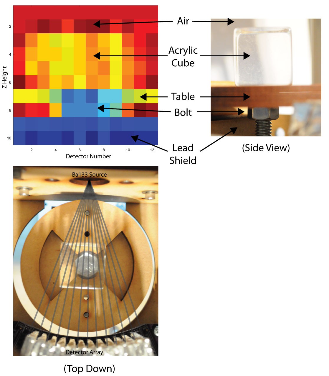
I decided to try to use a small acrylic cube as a test article, because acrylic appears reasonably absorptive to x-rays, and unlike the fruit and vegetables that I've been scanning, it doesn't decay. Above is an image constructed by measuring the absorption along 10 positions on the Z (up/down) axis, over about 50mm/2 inches of height. Here, on the bottom of the image, we can clearly see several features:
- Starting from the bottom, the lead shield, which blocks most of the high energy particles travelling from the Ba133 source towards the detectors, when the Z axis is at the lowest (homed) position. (High absorption, blue)
- Next, the metal M8 bolt used as a shaft for the sample table. (High absorption, blue)
- The MDF sample table (Medium absorption, yellow). The bolt is visible through the middle of the MDF (blue)
- The acrylic cube (low (red) to medium (yellow) absorption, depending on how much acrylic a given emission path has to travel through on the way to the detector)
- Air, at the top (very low absorption -- red).
All the important elements (shield, bolt, table, acrylic, air) are clearly visible and easily differentiated. The image might look a little unusual because (a) it's measuring absorption (like density) instead of the amount of light a given location is reflecting back, and (b) the image plane is cylindrical rather than flat, so that the distance from the source to each pixel on the detector array is constant -- so it's like the opposite curvature of a fish-eye lens.
A very successful image. Above, because of the extremely low intensity source, each pixel is the aggregate of about 15 minutes of exposure. The long integration time is to get a rough estimate of the actual absorption given the high rate of shot noise, which (at this integration time) appears to be in the neighbourhood of +/-20% -- so still quite large, but not impossibly so.
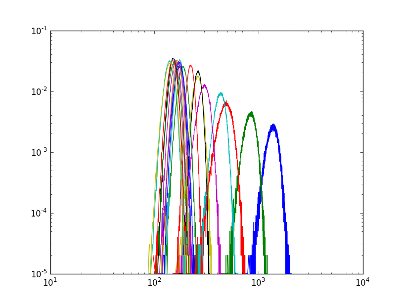
In spite of using some of the most precise opamps and high tolerance passives that are available, to my surprise, there is still a good deal of individual variation in the noise levels between each of the 12 detectors. This is a very important result, and answers a question I'd often had about the fantastic Radiation Watch Type 5 detector, used in the first OpenCT -- the detector is capable of detecting much lower energy levels by changing a single resistor value on the comparator, so why did they set the threshold so much higher? The answer is that setting the threshold very conservatively likely increases the manufacturing yield -- with the possibility for so much variation between units, the designer likely chose a safe value to ensure that >99% of their detectors would pass the QA process, at the expense of many of those detectors being less sensitive than they may ultimately capable of being.
By including the digital potentiometer in my design, I ensure that the detection threshold of each detector can be individually tuned to just above it's noise threshold, ensuring that each detector is at peak efficiency. From the cable of counts (above) for each of the 12 detectors at 10 different digipot settings, one can see that a uniform safe resistor value might have had the efficiency of each detector lowered by between 10-50%, meaning significantly longer integration times for the same signal. A definite win, when working at the extremely low signal-to-noise ratio of this system.
Ba133 emits over a wide range of energies, and the detector likely isn't detecting anything below 40keV, where noise is dominant. When performing the calibration procedure, I had had the secret hope that at very low digipot thresholds, where the noise level is higher (and many more false positives are detected), there would also be a higher number of lower-energy signal photons -- and that, by diving deep into the noise, one could tap detecting these lower-energy emissions for extra signal, and decrease the integration/scan times.
To investigate this, instead of recording the total number of detections over the entire 10-15 minute detection time, I record the number of detections over small (2 second) intervals over the 10-15 minute sample time, resulting in a list of 300-450 data points. Because shot noise is dominant in this extremely low intensity imaging, I use a statistical technique called bootstrap resampling to construct a probability distribution of showing likely values of what the actual absorption for a given pixel was. I'm hoping to use this to convert the tomographic reconstruction into an optimization problem and get away with shorter sampling times, but here I used it to estimate the amount of signal vs noise for given detector values. After an evening of tinkering, it looked like while there is definitely less signal when the threshold is raised, there doesn't appear to be more (easily identifiable) signal when the threshold is lowered -- so a simple calibration procedure of finding the digipot setting for each detector where the noise exceeds the background of ~2 counts per minute seems the simplest and most effective calibration procedure, right now.
Tomographic Sampling -- First, a simultation with a brain phantom
From classes in graduate school and my first postdoctoral fellowship, I know the basics of tomographic imaging -- but taking the concepts and translating them into a desktop hand-built scanner to collecting data to processing that data is a bit of an iterative learning experience for me, and a good experience to help solidify that knowledge, and fill in the murky areas. I hope others will find it as such, too.
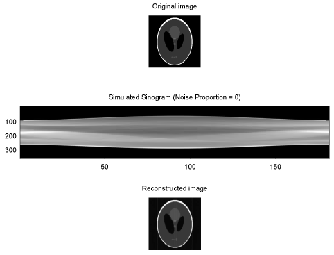
One of the best ways to do science and engineering is to predict what you expect to observe, and then actually observe that phenomenon, to see if your measurements match the predictions. For medical imaging, often one will simulate a scanner coupled with a reconstruction algorithm when using a "phantom", which is either simulated data (or an actual, simulated object, like a fake brain-like shape made out of acrylic). Above, we can see such a phantom, simulated in Octave (like Matlab, but open source) using the image processing toolbox. The phantom here is meant to very coarsely approximate a brain -- a roughly round head, with a few different oval structures inside.
In the simulated computed tomography scan above, we can see the original image (top), the simulated CT data called a sinogram, and the reconstructed image backed out from using the sinogram. The sinogram is an unusual image that's hard to visualize, but conceptually relatively straightforward -- imagine instead of taking a 2D absorbance image of an object (like an x-ray), you were to take a 1D absorbance image (one line from that 2D image) -- but to do this repeatedly, rotating the object at different angles, perpendicular to the axis that is being imaged. This is what a sinogram is -- a large set of 1D absorbance images, from different angles, which can be processed to produce a 2D slice of that object.
Where the above reconstruction simulates 180 images (taken by rotating the phantom by 1 degree increments), with about 300 detectors, and zero detector noise (i.e. perfect measurement), we can change these parameters to more closely approximate the OpenCT2, to determine what reconstruction quality we're likely to expect to observe.

Above is the same simulated phantom reconstruction, here imaged by rotating at 4.5 degree increments instead of 1 degree increments. 4.5 degrees was chosen as it approximates what the OpenCT2 could scan within about 8 hours, assuming 15 minutes of measurement per angle. Here, we can see that reducing the angular resolution has a small but noticeable effect on the reconstruction image quality (bottom).
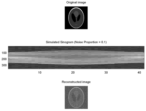
Unlike a normal CT scanner, the extremely low intensity source on the OpenCT2 means a very high amount of shot noise, even at a 15 minute integration time. The shot noise at this level looks to be somewhere between +/-10% to +/-20%, so I simulated two noise levels. Above is 4.5 degree samples with the sinogram distorted by +/-10% Gaussian distributed noise. We see this dramatically reduces the reconstruction quality.
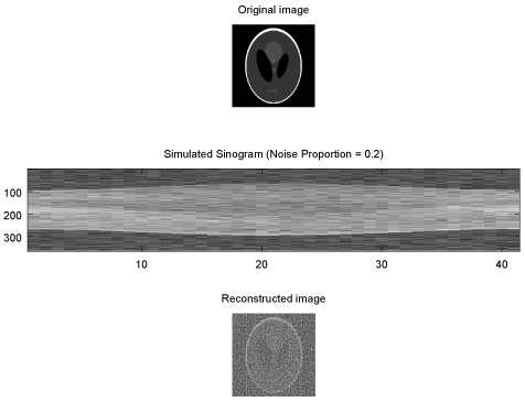
Similarly, above, at +/-20% Gaussian noise, the image quality is severely reduced -- we can make out the overall shape of the phantom, as well as the two large dark structures, but the smaller structures are no longer easily visible.
Simulating the Acrylic Cube
Since the first tomographic scan is of an acrylic cube, here I've run the same simulations on a phantom cube. First, the zero noise simulation:

Note how the sinogram appears to oscillate, from entirely solid (x=0,20,40) to solid in the middle while less intense at the outset (x=10,30). This is as a result of the rotation of the cube -- when the cube is face-on towards the simulated detectors, the absorption is approximately equal(x=0,20,40), where as when the cube is rotated at a 45 degree angle (x=10,30), the absorption of the center detector will be significantly increased (as the x-rays now have to travel on a diagonal across the cube -- the maximum amount of cube to travel through), where as the detectors along the edge have little to cube to travel through (so their absorption is less).
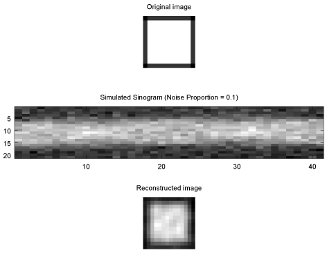
Adding in +/-10% of simulated Gaussian noise distorts the shape of the cube somewhat, and certainly it's uniformity, but we're still able to make out the overall shape.
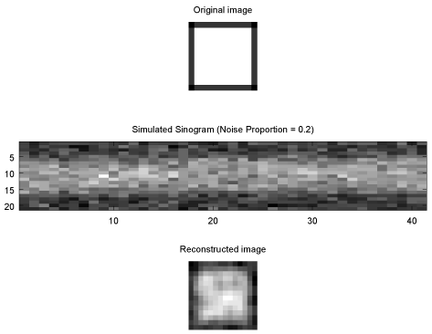
And above, at +/-20% of simulated Gaussian noise on the sinogram, the both the shape and uniformity start to become distorted, but we can still make out the overall shape.
Finally, real data!
I collected the first tomographic data of the cube by setting the Z axis to the middle of the cube, and leaving it to collect data at 4.5 degree angles overnight, with 15 minutes of integration time per angle.
The simple reconstruction method above doesn't perfectly match the OpenCT2 setup, with detectors densely populated over a small number of angles (about 60 degrees of angle), rather than distributed across 180 degrees. To take this into account, I've zero-padded the outside angles of the sinogram. This simple reconstruction also won't match in several other ways, so it won't be a perfectly faithful reconstruction, but it'll be an okay first pass. Let's have a look:
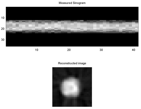
That is definitely a cube! This is a reconstructed tomographic slice right through the center of the acrylic cube, and looks very reasonable. This is also the first tomographic reconstruction from the OpenCT2, which is very exciting!
Simulated Checks/Controls
Since I'm still an amateur at tomographic reconstruction, and learning as I go, I decided to run several quick checks to simulate what a reconstruction might look like under two different circumstances, to ensure that the cube-like nature of the reconstruction is due to real measured data, and not an artifact of the algorithm, or wishful subjective interpretation. The first check is for a uniform sinogram, zero padded at extreme angles, as above:
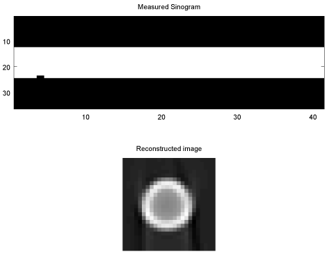
Were the data to be roughly uniformly distributed across all detectors, the reconstruction would look as it does above -- essentially a slice of a cylindrical pipe, with walls, and a less dense interior. This doesn't look like a slice of a cube -- so far, so good!
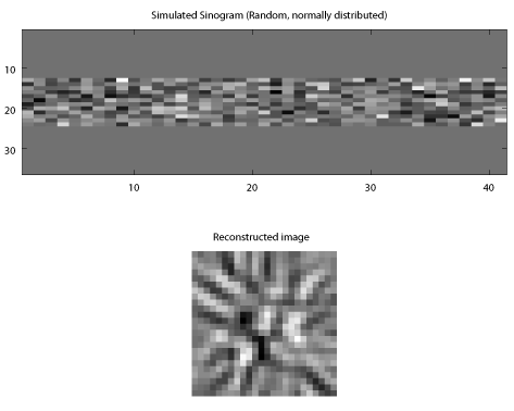
The next check is a random baseline, here with normally distributed random values. This definitely doesn't look like a slice of a cube (or, like anything but noise, to me). Still looking good!
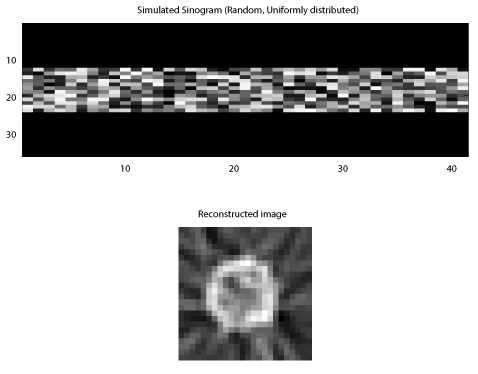
And finally, another random baseline, here with uniformly distributed random values. This looks like a noisy hollow cylinder, much like the first uniform baseline, though the right side does subjectively look a little straight -- so while it may have some square-like properties, it's definitely much more similar to the two other controls, and substantially different from the measured data.
Success!
And so, finally, a year after starting this build, there's some success -- the first (admittedly reasonably noisy) tomographic reconstruction, from an extremely low intensity radioisotope source, and a bench-built photon-counting imaging array. Very cool!
From here, it seems that a beneficial next step would be to better characterize the integration times required for a given reconstruction quality by constructing a series of laser cut acrylic phantoms that simulate different shapes, some with internal structure, and performing tomographic scans of these objects.
Mechanically, the entire unit is now self-contained, and needs a number of small but significant finishes (like the outer cylindrical cover) to happily and attractively sit stand-alone on the desk, and run for extended durations.
Discussions
Become a Hackaday.io Member
Create an account to leave a comment. Already have an account? Log In.
Are you going to be able to get better noise immunity by running longer?
So, like, leaving it running while you go on vacation for a week or two? :p
Are you sure? yes | no
Yes -- measurement uncertainty decreases with the square root of the number of measurements, so doubling the number of measurements will decrease uncertainty by a factor of sqrt(2) = 1.4, four times as many measurements will decrease uncertainty by a factor of sqrt(4) = 2, 9 times the measurements = 3, 16 times the measurements = 4, and so on. This can be seen graphically in the histogram of detector performance I included at the bottom of this post:
https://hackaday.io/project/5946/log/20074-assembling-and-characterizing-the-modular-detector-rev1
But rather than increasing the integration time to get a better picture, the more interesting science is in using clever statistical techniques to built better reconstructions with fewer samples. In the context of medical imaging, this is usually explored in the context of lowering the radiation dosage. I really know only the basics of computed tomography (again, only a few classes, and an avid interest), and relatively little about low dose methods, so it'll take a bit of reading before I know what the modern techniques for working with shot noise are. Intuitively it seems that with photon counting you could use the likelihood distribution to solve an optimization problem to find the most likely reconstruction, even in very noisy cases, and I'm sure someone has formalized this more.
Are you sure? yes | no