 Ted Yapo
@peter jansen had an interesting take on my earlier Monte Carlo simulations exploring the effects of scramble-winding coils vs neatly layered windings. He wondered how the angle of the field was perturbed by the random windings - my previous simulations had all examined just the magnitude of a single component of the field (in the axial direction). It turns out that the framework I'd put together for the earlier analysis just needed a little tweaking to examine angles.
Here's a representation of the field vectors at each point, Pk, in space:
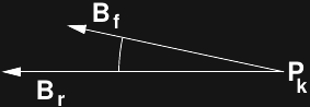
Br is the field vector in the center of the reference coil - in this case, a 40mm radius Helmholtz coil with two single-loop windings, while Bf is the field vector for a particular sample of scramble-wound coil. The angle between the fields can be calculated by:
I already had the code to draw contour areas based on thresholding scalar values, so I substituted this angle for the previous magnitude criterion. As before I ran 10,000 randomized simulations of scramble-wound coils, then used symmetry for an equivalent 40,000 samples. I'll skip presenting the individual images here, and jump right to the probability distributions:
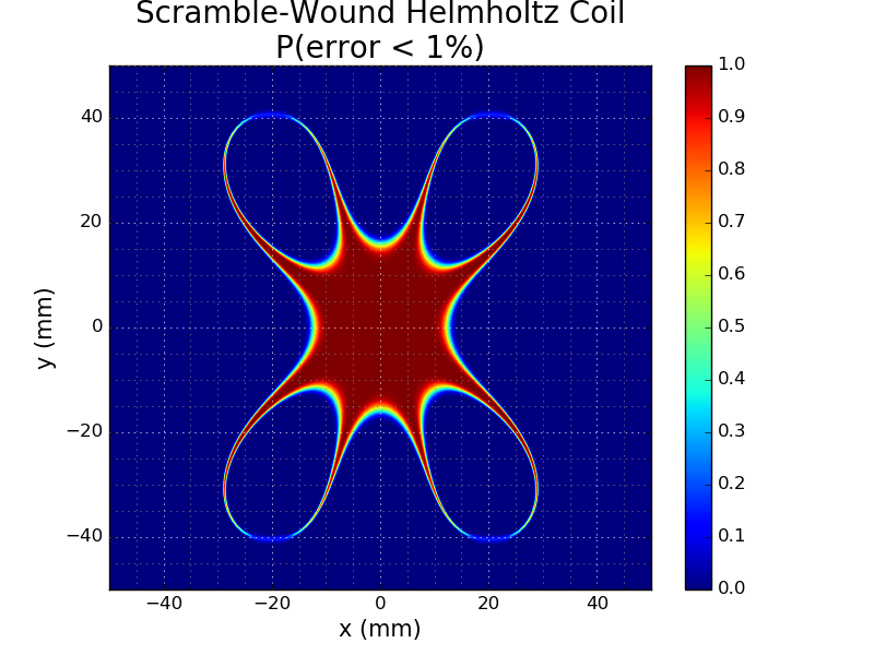
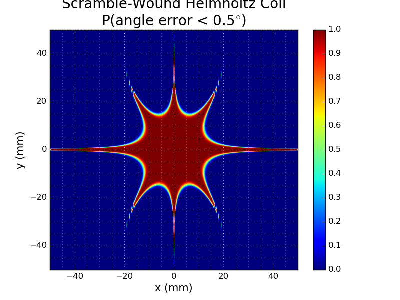
The left image is the magnitude distribution from before: the colors indicate the probability of achieving less than 1% error in the x-axis component of the field. On the right, we see the new analysis: the probability that the angle of the generated field vector is within 0.5 degrees of the reference field direction (equivalent to a 1-degree wide cone around the reference). Note that the reference here is the field in the center of the reference coil; not the field at the the corresponding spatial point in the reference field. The shapes of the level curves look complementary or "dual" in some vague but satisfying way.
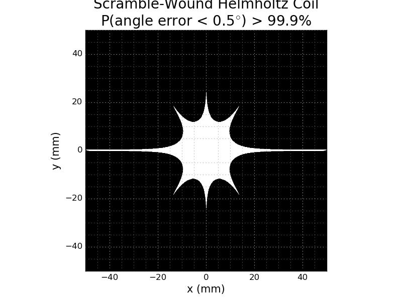
Like the magnitude version, the angle plot is difficult to read; to get a better view, I again thresholded the probability. This plot represents the area in which you have a 99.9% chance of the field being within 0.5 degrees of the reference (I have to figure out why the title text is getting cut off):
Of course, you might care about both magnitude and direction. Here's a similar pair of plots for the logical and of the conditions: P(magnitude error < 1% and angle error < 0.5 degrees):
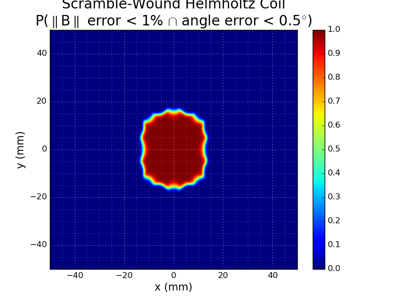
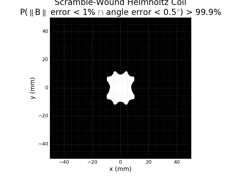
In this plot, I've used the total magnitude of the B field, instead of just the x-component magnitude as in the others. The right image is again thresholded at 99.9%. The thresholded region encloses a sphere of 15mm diameter, just a little smaller than the 16mm using the magnitude criterion alone.
I'm planning to add a version of this code to the GitHub repository, but I have to clean it up a bit, and make a decent API for the two pieces. Another thing to add to the to-do list :-)
Discussions
Become a Hackaday.io Member
Create an account to leave a comment. Already have an account? Log In.