Unit-to-Unit Heading Accuracy Variation

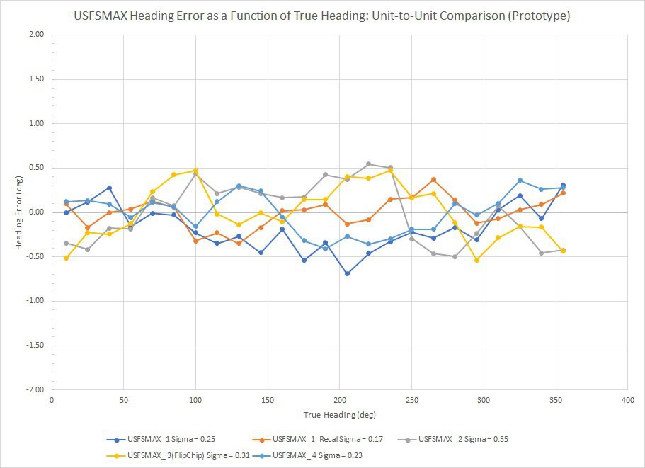
In my last log entry I mentioned the need to characterize the unit-to-unit variation of heading accuracy among professionally manufactured MAX32660 motion co-processor boards. We are still waiting for delivery of our initial production runs, so in the mean time I decided to characterize the four prototype units I had on-hand. I used the same precision goniometer, calibration method and experimental procedures described in my previous log entry. The plot below shows heading error as a function of heading.

Results from a total of four units are included in this plot with two data sets from "Unit 1" representing two different trials of the calibration method. The RMS heading error ranged between 0.17 and 0.35 degrees. If anything we would expect professionally manufactured units to have more precise location/alignment of the MEMS sensor chips on the circuit board than these hand-built prototypes. So if placement of the accel/gyro and magnetometer chips effects post-calibration heading accuracy, we might potentially see less unit-to-unit heading accuracy variation on production units than what I have measured here. However, the nature of the 24-point tumble calibration described earlier should robustly correct accel/gyro/mag misalignment. So I would expect these results to be a representative sample of the MAX3260 motion co-processor's heading accuracy capability. I will perform similar measurements on a sample from our first run of production units when they arrive early in 2020.

On-Board Real-Time Hard Iron Error Correction

Throughout the slate of heading error characterizations I have performed, I noticed that heading error performance degrades slightly when the magnetic environment differs from the exact calibration conditions. This effect is not gross but is more like degrading from ~0.26 to ~1 degree RMS heading accuracy. This illustrates a typical complaint regarding IMU calibration: The stellar results generated during calibration on the test bench are seldom translated to the real performance in the field. Analysis of the heading error plots showed that the additional error is hard-iron-like in that it has a period of 360 degrees. This means the magnetometer response surface is still spherical but is displaced from the origin.

The heading error results shown above indicate that the suite of MEMS sensors we are using  (LSM6DSM and LIS2MDL) are stable enough to deliver ~0.26 degree RMS heading accuracy... So degrading to ~1 degree by incidental changes in the IMU's local environment should be correctable, especially since the additional error takes the form of a hard iron offset (the easiest to estimate and correct). The MotionCal (Freescale) magnetic calibration algorithm embedded in the MAX32660 is quite capable of dealing with this additional incidental hard iron error but it is too computationally intensive to run in parallel with the main AHRS fusion filter in real time.

Instead of just saying, "Oh well, such is life..." I decided to investigate the possibility of a simple, computationally efficient method of fitting a sphere to the locus of run-time (Mx, My, Mz) data points and extract estimates of the residual hard iron offsets. I found this reference which presents a practical embodiment of a method for geometrically fitting the "best sphere" through a 3D ensemble of data points. Upon examination, I particularly liked this method because 1) It is analytic and does not need to be solved iteratively and 2) Adding data to the point ensemble to be fitted only results in using more memory without increasing the computational load on co-processor MCU. The center point and radius of the best-fit sphere are calculated from a set of running sums that are cubic in X and Y. Executing a spherical fit after adding a new (Mx, My, Mz) data point consists of:

• Calculating the necessary cubic and quadratic terms from the Mx, My, Mz data
• Adding new terms to the running cubic, quadratic and linear term sums
• Using the running sums to calculate the new center point and radius estimates by simple algebraic manipulations

So the total computational load is fairly light and is the same for the first and Nth data points.

I tested the efficacy of this approach by:

• Programming the analytic sphere-fitting method on the host MCU 
• Subtracting the sphere-fit center point coordinates from each (Mx, My, Mz) data point
• Programming a duplicate AHRS fusion filter on the host MCU to reproduce the Euler angles with the hard-iron-corrected (Mx, My, Mz) data

Using this method I can generate the USFS max heading solution under the influence of a stray hard iron field and simultaneously simulate the sphere-fit-corrected version. Initial tests showed that the real-time sphere fit method is quite capable of neutralizing incidental hard iron effects. To prove the point, I purposely attached a small rare-earth magnet to the USFSMAX calibration/test fixture to impose a gross hard iron offset and then:

• Tumbled the test fixture briefly in three-space to populate sphere fit arrays with valid data and generate the hard iron corrections in-situ
• Characterized the heading-dependent heading error curves for the corrected and uncorrected cases simultaneously

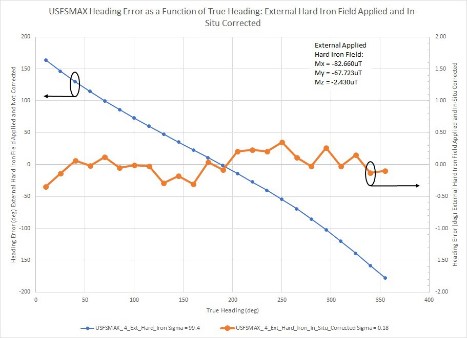
The applied hard iron offsets estimated from the spherical fit were Mx = 82.660uT, My = -67.723uT and Mz = -2.430uT. These components are actually quite large, as the geomagnetic field is nominally ~50uT. The blue curve (Left-hand axis) shows the heading error of the uncorrected USFSMAX motion co-processor AHRS solution under the influence of the applied hard iron offsets. The hard iron interference is so bad that the indicated heading is nearly constant, only ranging between 141.5 and 167.1 degrees in a full 360 degree rotation. The corresponding RMS heading error was 99.4 degrees. The bold orange curve (Right-hand axis)  shows the simulated corrected AHRS solution generated simultaneously on the host MCU. The RMS heading accuracy recovered to 0.18 degrees, essentially identical to the immediate post-calibration value.

I believe this is an important result. This real-time, in-situ method of fitting a sphere to the (Mx, My, Mz) data ensemble allows us to neutralize the degradation in heading accuracy performance that often occurs between calibration on the test bench and deployment out in the field. My next step will be to program this analytic sphere fitting method and associated infrastructure into the USFSMAX standard firmware. There will be a significant amount of experimentation required to learn how to best manage/filter which points are included into the sphere-fitting (Mx, My, Mz) data ensemble... And when to clear the data buffers and start over. But these initial results show there is a straightforward path to follow.