 CheeenNPP
Analog Lorenz Attractor Computer

1. The Origin of Analog Computer
One of the main purposes of analog circuits is to solve mathematical problems, such as building a circuit corresponding to a nonlinear differential equation and analyzing the phase plane characteristics of it by observing its output voltage with an oscilloscope or analog plotter. I will take a famous nonlinear differential equation, the Lorenz Attractor, as an example, and show the whole process of solving it with an analog circuit.
2.Lorenz Attractor
The Lorentz attractor is a set of equations describing the dynamical behavior of the atmosphere, which reveals the chaotic phenomena contained in meteorological changes and is known as the "butterfly effect". The Lorentz attractor consists of three nonlinear differential equations:

Among them, sigma, b and r are the three constants that determine the characteristics of the system, commonly taken as sigma = 10, r = 28 and b = 8/3. Before building the analog circuit, we can simulate it with software to understand some basic characteristics (sounds a bit strange~~). The software used is Octave, and the Lorentz attractor function is declared in lorenz.m, where x is a three-dimensional vector set, and x(1), x(2), and x(3) represent x, y, and z in the original set of equations, respectively, while a scale factor k is added for further usage.
% Lorenz.m

function dx = lorenz(x, s, r, b, k)
    dx = zeros(3, 1);
    dx(1) = k*(s*(x(2) - x(1)));
    dx(2) = k*(-x(1)*x(3) + r*x(1) - x(2));
    dx(3) = k*(x(1)*x(2) - b*x(3));
end
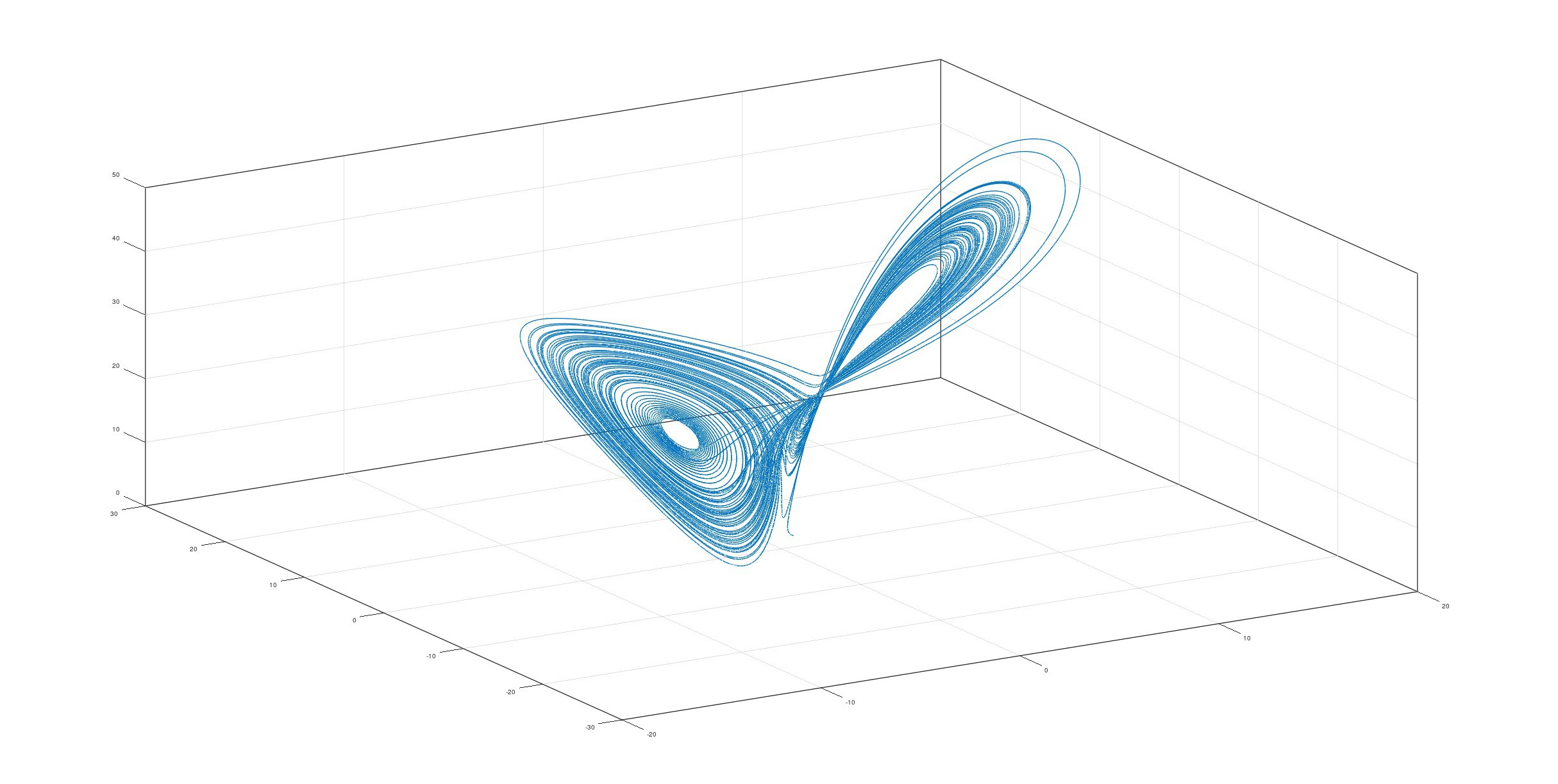
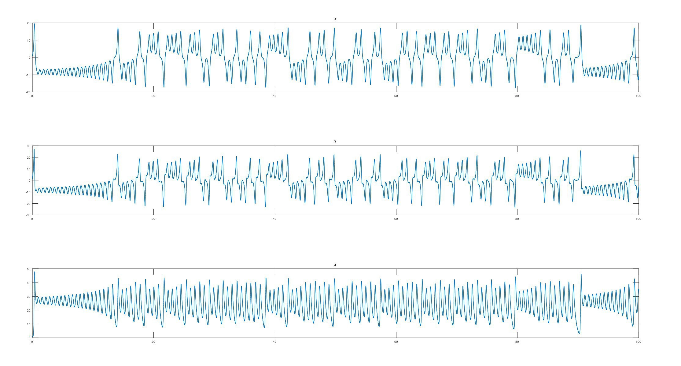
The lorenz function is called in test.m and solved numerically. Here the fourth-order Runge-Kutta method is used and the initial values of the equations are set to (1, 1, 1). Finally, the trace of x is presented in three and one dimensions, respectively:
% test.m

clc; clear all;

dt = 1e-3;
t = 0 : dt : 100 - dt;

s = 10;
r = 28;
b = 8/3;
k = 1;

x = zeros(3, length(t));
x(:, 1) = [1; 1; 1];

for tn = 1 : 1 : length(t) - 1
    k1 = lorenz(x(:, tn),           s, r, b, k);
    k2 = lorenz(x(:, tn) + dt*k1/2, s, r, b, k);
    k3 = lorenz(x(:, tn) + dt*k2/2, s, r, b, k);
    k4 = lorenz(x(:, tn) + dt*k3,   s, r, b, k);
    x(:, tn + 1) = x(:, tn) + dt/6*(k1 + 2*k2 + 2*k3 + k4);
end

figure;
plot3(x(1, :), x(2, :), x(3, :), '-'); box on; grid on; drawnow;

figure;
subplot(3, 1, 1); plot(t, x(1, :)); title("x");
subplot(3, 1, 2); plot(t, x(2, :)); title("y");
subplot(3, 1, 3); plot(t, x(3, :)); title("z");
The simulation results are shown in the following figure:
3.How to Design an Analog Computer
How can this set of equations be "translated" into an analog circuit? This is illustrated by a diagram:
In analog circuits, the most convenient circuits used to perform calculations are those designed based on inverting amplifiers, which are simpler in form than non-inverting amplifiers and also avoid distortion and noise from common-mode operation, which was particularly important in the early years of op-amp development.
In the first step, determine the implementation of the various operations as:
- Integral: use the inverting integrator circuit, but temporarily discard the resistor, which is equivalent to integrating the input current and multiplying by -1.
- Multiplying by -1: use the inverting amplifier and set the two resistors with the same value.
- Addition: use current summation instead of voltage, so the form is simpler.
- Multiplying by a constant k: use a resistor with a resistance of 1/k, the voltage across it is converted into a current and output as a result.
- Multiplication: implemented using a dedicated voltage multiplier.
In the second step, the integrator is cascaded with the inverting amplifier, and the output of the integrator is set to -x, the output of the inverter is x, and the input of the integrator is dx/dt. Then calculate the equivalence of dx/dt and input it at dx/dt. The x and -x signals needed in the operation are obtained from the above output. y and z signals are obtained in the same way. The signal flow diagram can be drawn in this way.
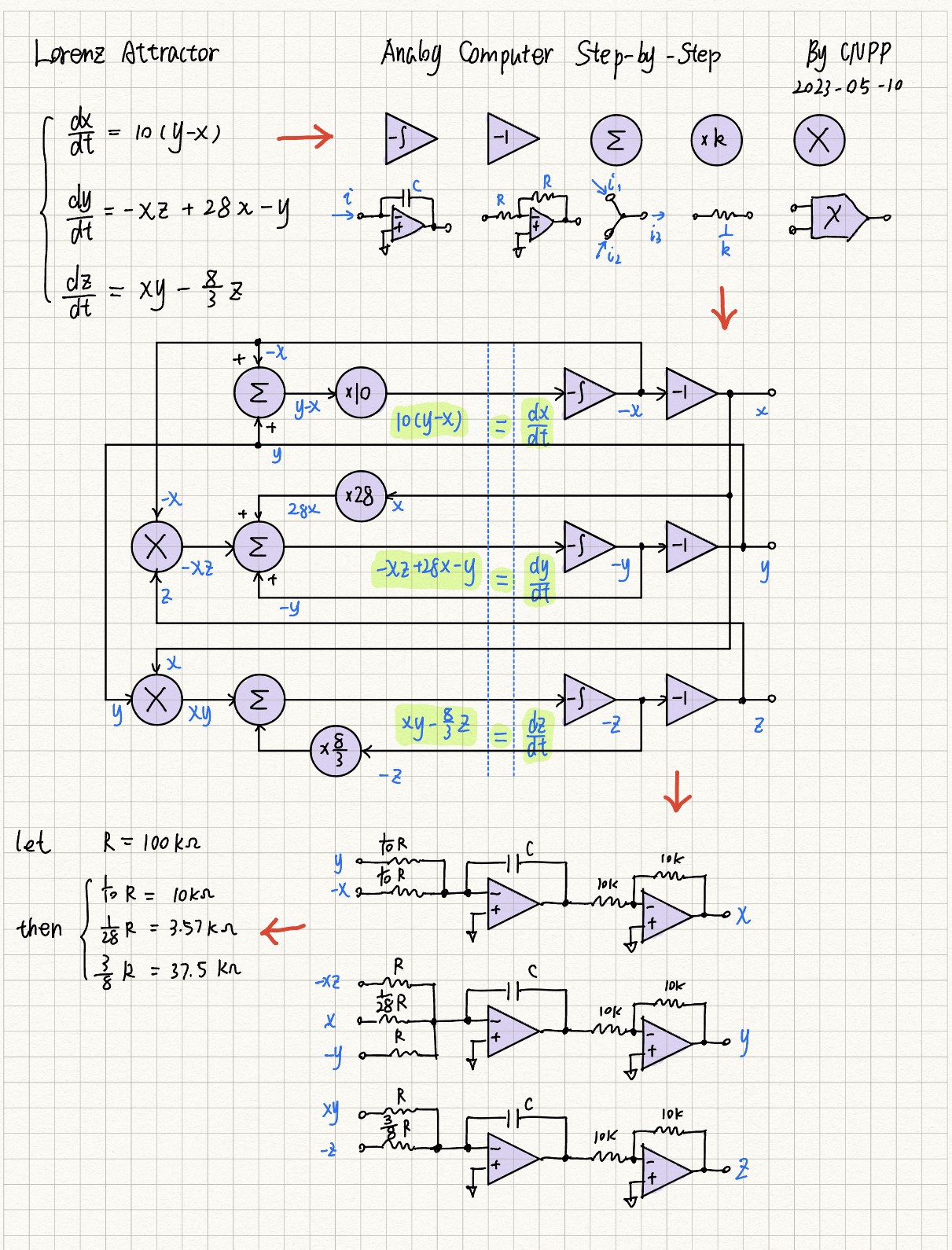
In the third step, the signal flow diagram is transformed into a circuit by combining the operational circuit designed in the first step. The resistance value of the inverting amplifier is taken to be the commonly used 10kOhm, the integral capacitor value of the three circuits is kept the same, and the proportional resistance value is set to be R multiplied by each proportionality factor. The actual values of the required resistors are 10kOhm, 100kOhm, 3.57kOhm, and 37.5kOhm. Subsequently, the corresponding signals are connected to each other. Here, the output to input connection and multiplier are omitted.
Finally, we can check the correctness of the calculation circuit:

Moving the coefficients before the RC to the variables:

Extracting the common factorization and combining the integral:

Derivative for t on both sides:

As can be seen, the above set of equations for the analog circuit has an additional factor 1/RC compared to the original set of Lorentz attractor equations. This coefficient is proportional to the rate of change of the variable with respect to t, which can be interpreted as the "speed of the operation", and can be observed by changing the parameter k in the previous Octave simulation code.
4.Simulation
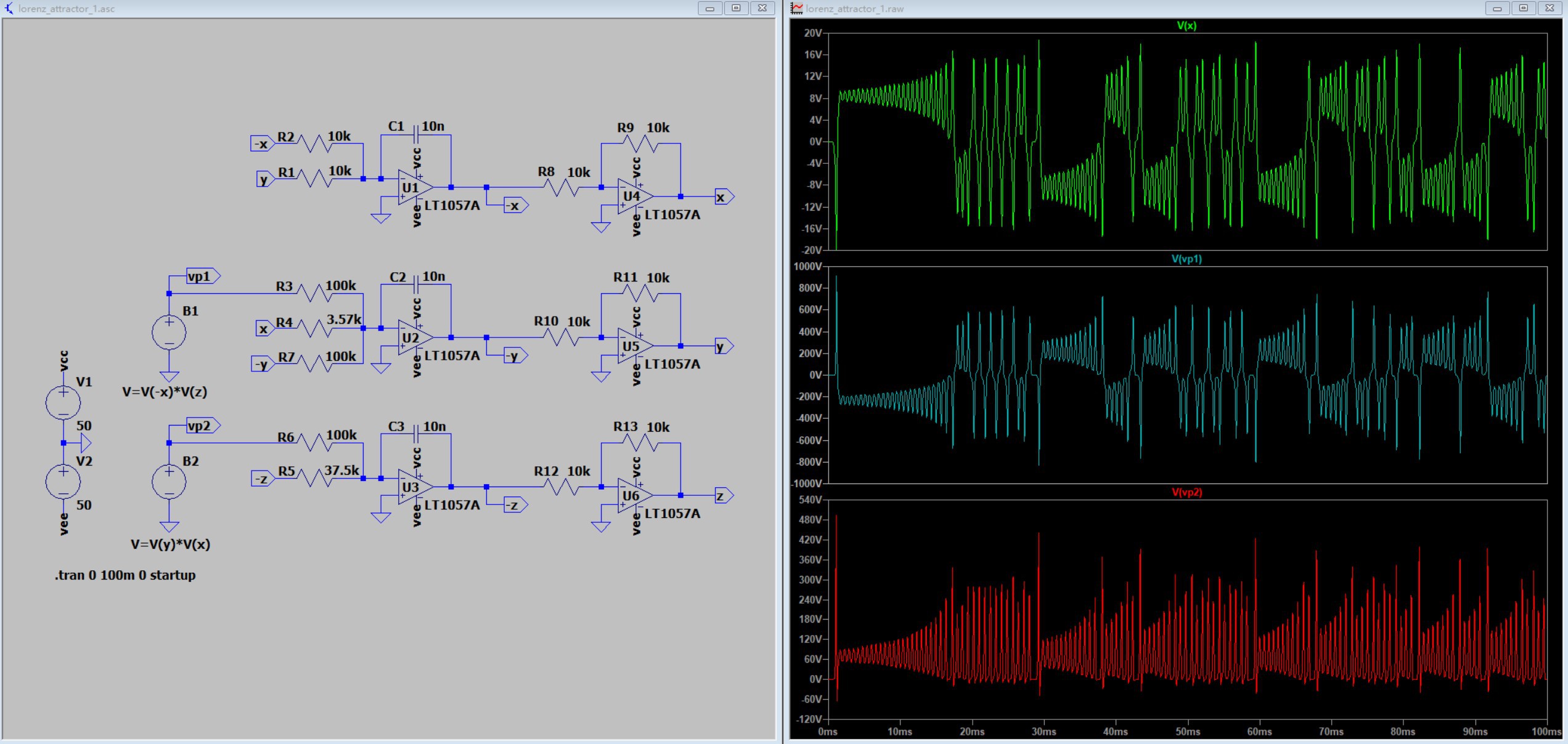
The Lorentz attractor circuit is simulated in LTSpice, using an arbitrary voltage source (bv) instead of a multiplier, the value of the integrating capacitor is temporarily taken as 10nF, and the op-amp is selected as LT1057 or a precision medium-speed (GBW around 10MHz) part with similar parameters, and the simulated waveform is shown below.
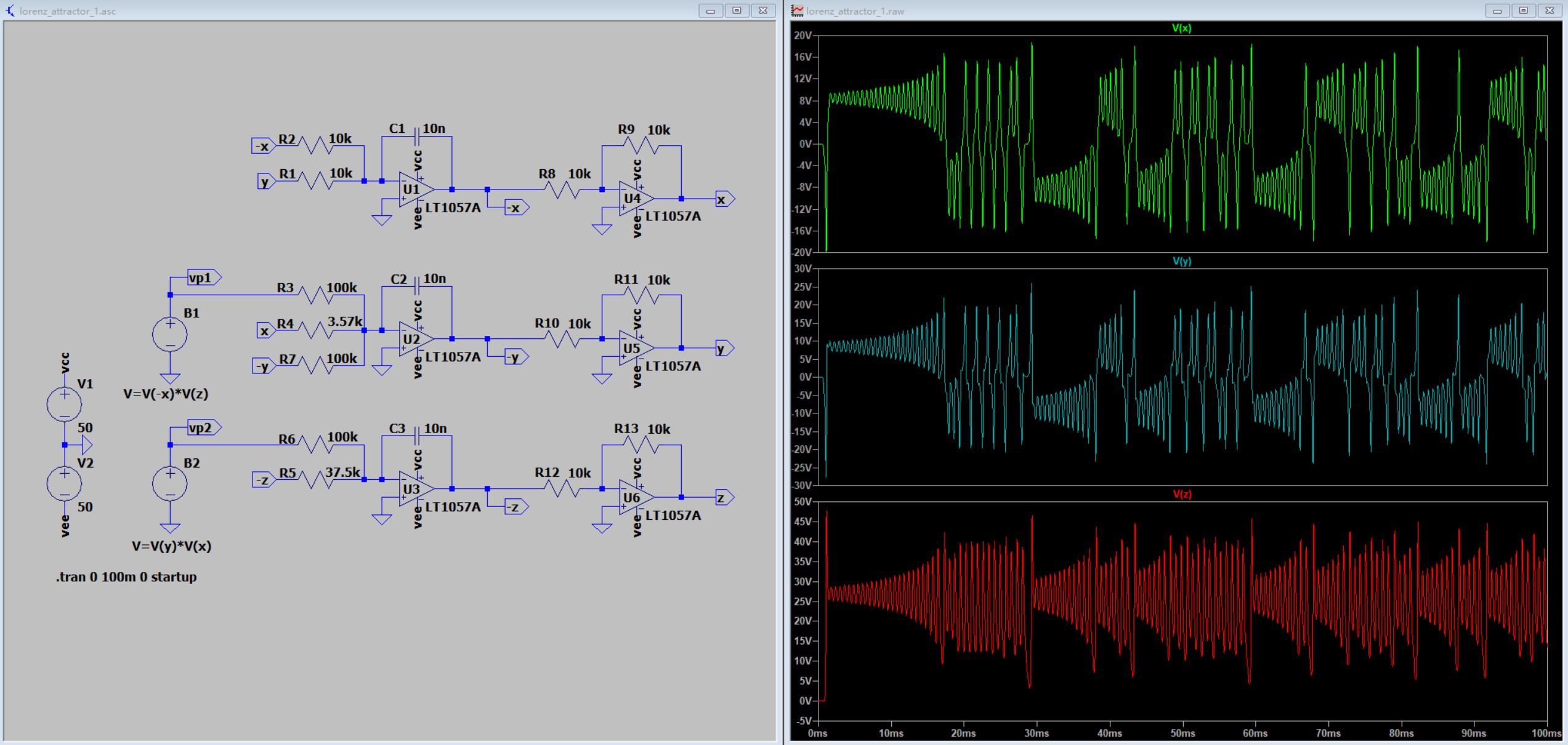
Observing the waveform as well as the amplitude, and comparing it with the simulation results of Octave above, it can be seen that the simulation circuit accurately accomplishes the solution of the nonlinear system of equations. During the circuit simulation, some important issues can also be identified:
- The resultant amplitude of the original Lorentz attractor equation solution is close to 50 at the highest, so for direct simulation, the supply to the op-amp needs to be set to at least +-50V, otherwise the simulation results will be incorrect. However, +-50V is obviously higher than the supply voltage that the LT1057 op-amp can withstand, but LTSpice does not limit this and still yields correct results. Also, when making the actual circuit, it is not realistic to use such a high supply voltage and high voltage op-amp, so the circuit has to be modified for optimization.
- When the signal is large, it becomes even more frightening when processed by the multiplier. Observe in the figure below that the multiplication outputs vp1 and vp2 have voltages even close to a thousand volts. So when using a multiplier, pay special attention to the range of the input and output signals. Usually the transfer function of the multiplier chip is Z=XY/10 or Z=XY/k with k adjustable, etc. This is designed to prevent the output signal from being too large.
The above two analyses allow us to optimize the circuit. Firstly, by testing it was found that the amplitude of the operation result can be reduced by inserting the attenuation coefficient d (d>1) after the two multiplication operations of the equation:
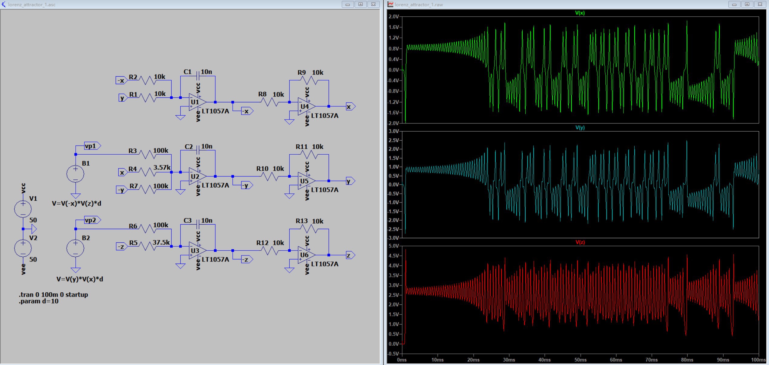
In taking d = 10, the output signal becomes 1/10 of the previous one, so that it stays within the common operating voltage range of the op-amp. The operation of multiplying the multiplier output by 10 can be converted to reduce the resistance of the proportional resistor connected to the multiplier output to 1/10 of the original value, i.e., from 100kOhm to 10kOhm.
After the change, the output of the multiplier is then examined to see if it is too large:
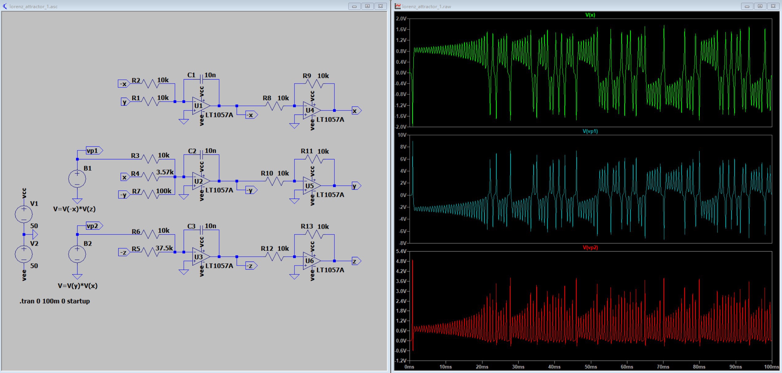
As seen in the above figure, the maximum output of the multiplier is still close to 10V. To reduce it, the multiplier can be configured in the form of Z=XY/10. Also, to compensate for this change, the proportional resistance of the multiplier output connection needs to be reduced by a factor of 10 again, i.e., from 10kOhm to 1kOhm, as shown in the following figure:
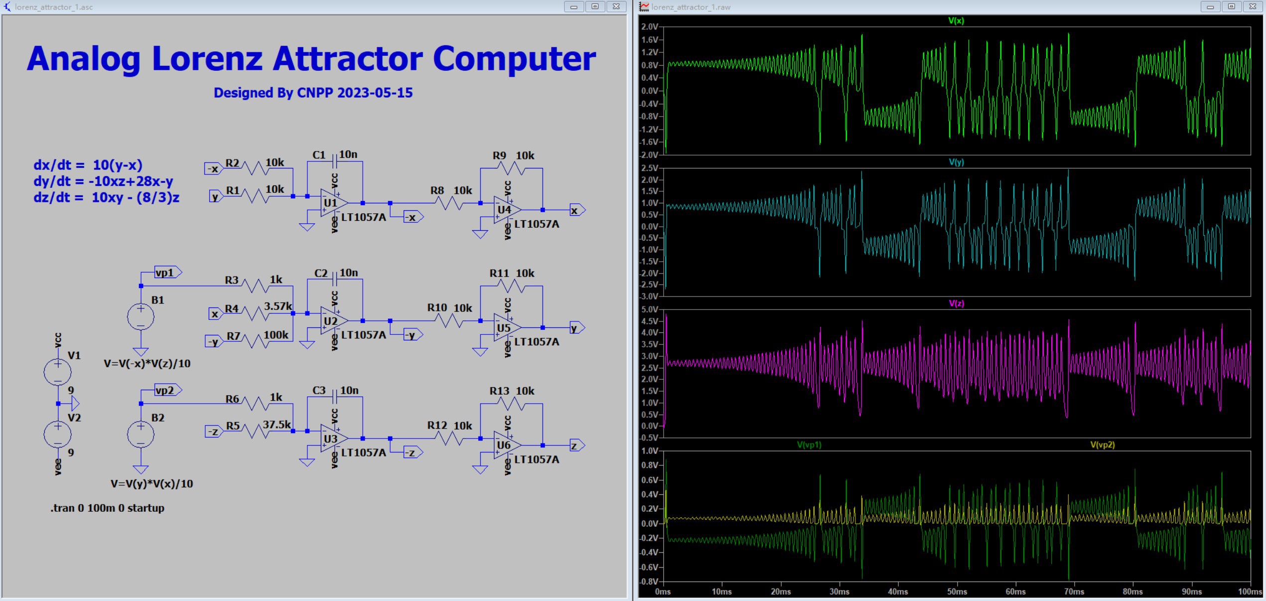
At this point, the optimization is complete and the entire system can also operate normally with a +-9V supply. If you want to further reduce the supply voltage, you can follow the above analysis.
5.Hardware Implementation
The most critical part of the whole circuit is the analog multiplier. It needs to have a high dynamic range (able to handle input signals within 5V) sufficient linearity and appropriate bandwidth (within 1MHz). The more common precision low-frequency multipliers are the AD633 and MPY634, but they are very expensive (the AD633 is positioned as a low-cost multiplier, but still sells for a lot of money). Other options are the ancient MC1495 multiplier (which I don't have on hand at the moment), as well as modifying the MC1496 for use as a multiplier (the MC1496 is a Gilbert-type mixer with a small input dynamic range and low linearity, with the advantage of higher bandwidth) or modifying a V/V linear voltage controlled amplifier such as the LMH6503 for use as a multiplier, etc. In short, there are many ways. And I happened to find a cold analog multiplier chip NJM4200 at a thrift store:
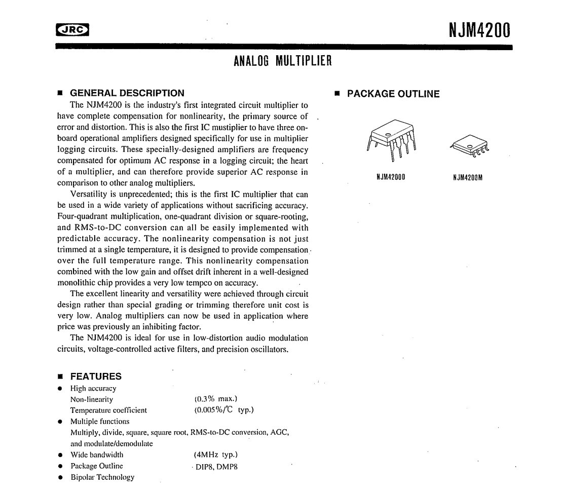
It uses a log-exponential conversion structure that performs a multiplication operation on the current. By configuring external resistors, it is possible to obtain an input dynamic range of up to 10V, while the disadvantages are the very high number of external resistors required and the drift of the internal op-amp that affects linearity.
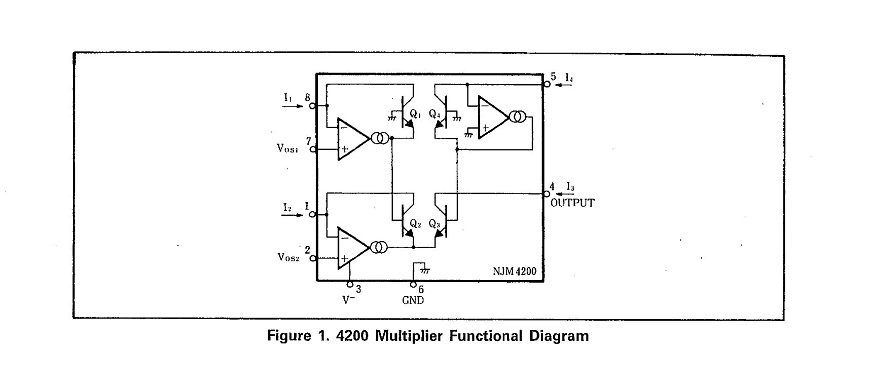
The configuration process for the NJM4200 is tedious and requires consideration of the input signal range and the need to add an op-amp for I-V conversion. A more easy-to-use connection is given below:
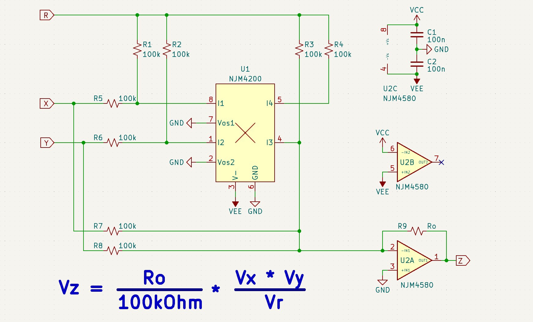
If a transfer function of Z=XY/10 is required, Ro can be taken as 100kOhm and Vr can be connected to a reference voltage of 10V; or Ro can be taken as 10kOhm and Vr can be connected to a reference voltage of 1V. In addition, Ro or Vr can be set to be fine-tunable for testing.
For operational amplifiers, you can choose TL082, LT1057, NJM4580 and other models with high input impedance and speed in the audio class. After the selection and the values were determined, I completed the circuit on the cavity board as follows:
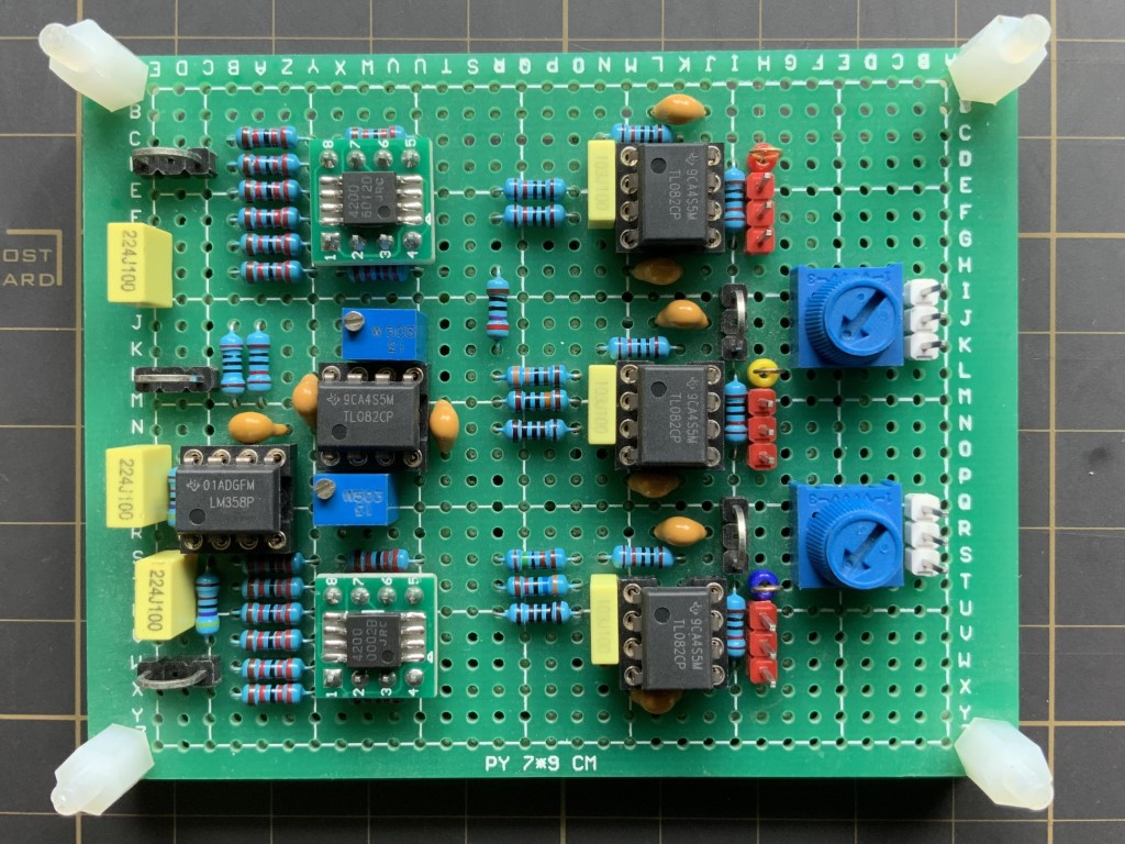
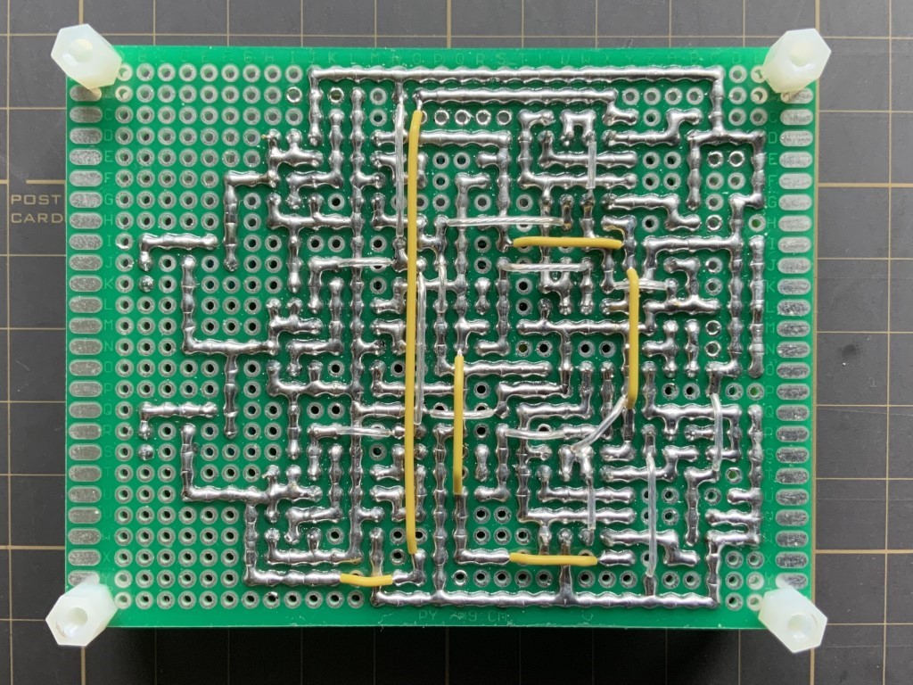
Using the X-Y mode of the oscilloscope to observe the waveform at the output port of the circuit, the phase diagram of the Lorentz attractor can be observed by different combinations of:
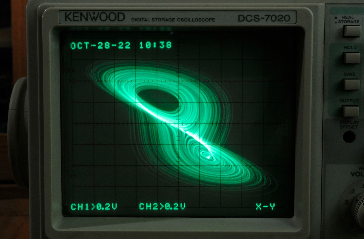
X-Z
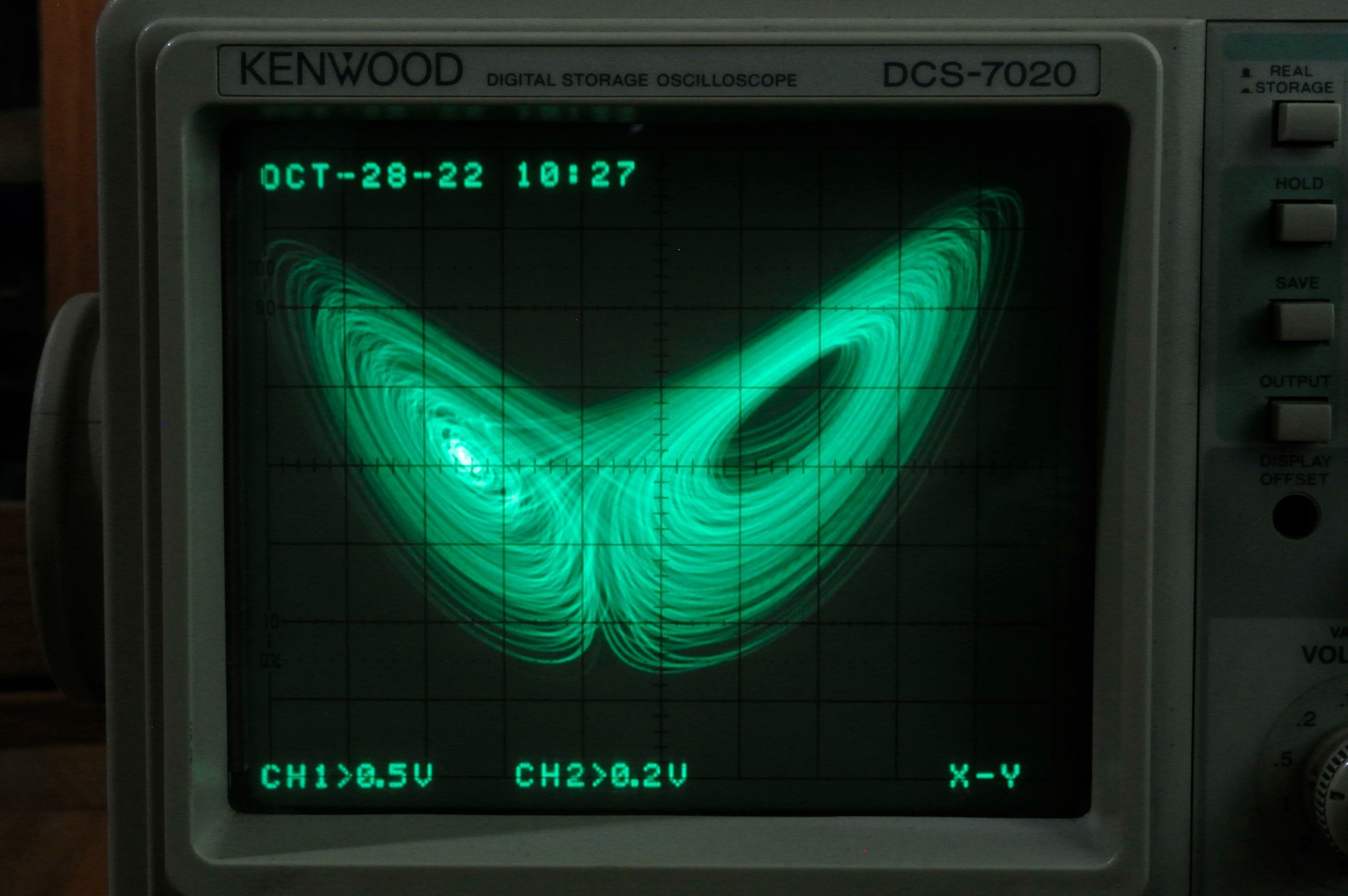
X-Y
Y-Z
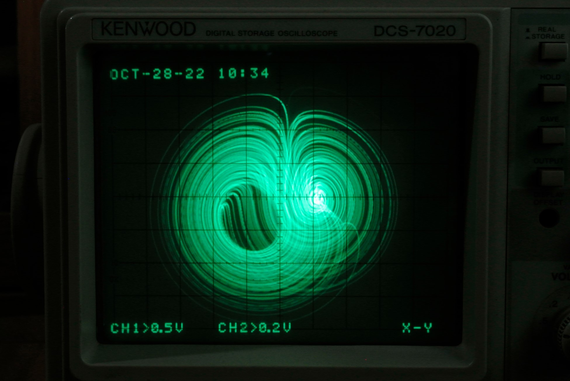
This set of images was obtained using the camera's long exposure, with the phosphor afterglow of the analog oscilloscope, which has a very illusory and ethereal beauty, just like the elusive chaos implied by the Lorentzian attractor.
6.Postscript
This is my first attempt at a vintage analog circuit, and I didn't expect such wonderful results. Currently, I have started a new journey of exploring analog circuits to solve difference equations, so I look forward to seeing you next time.