 Sebastian
Background and motivation
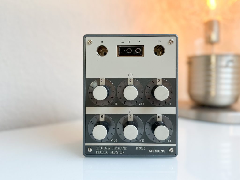
In 2021/2022 I designed a DC electronic load that would be more capable, but also much more complex than the usual DIY solutions. However, after building a working breadboard prototype of the analog circuitry with 12 ICs including multiple precision and dual opamps, I thought that it might be better to start with a smaller project that would allow me to gain a lot of experience and write much of the non-application specific code that I could use later on for the digital part. Also, at the time I was looking for a decade resistor box to add to my lab. And this is how I started working on a programmable decade resistor, a pretty specialized tool for niche applications.
Introduction
A programmable resistor is a electronic device whose electrical resistance can be adjusted typically through digital signals. Programmable resistors are available in form of integrated circuits (often referred to as digital potentiometers) as well as stand-alone devices/expansion cards. There are many different applications, each with their own set of requirements e. g.:
- programmable gain amplifiers
- sensor emulation
- hardware-in-the-loop simulation (detailed explanation below)
- calibrators
- prototyping
Basic concept
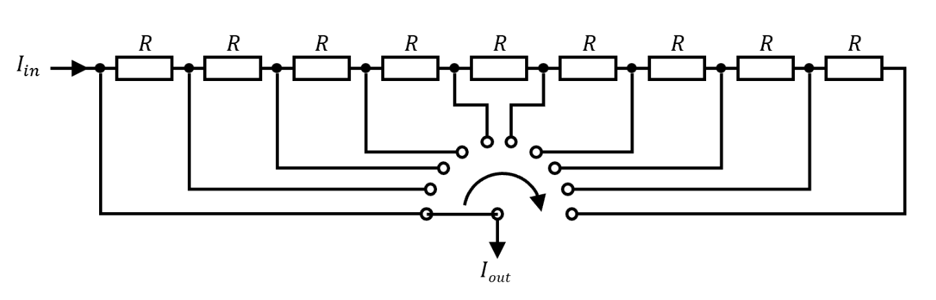
The programmable resistor closely follows the main principle of resistor decade boxes: connecting multiple devices (“decades”) in series, with each of the devices having a settable resistance of 0 Ω, 1 ⋅ 10n Ω, 2 ⋅ 10n Ω, 9 ⋅ 10n Ω, where n specifies the decade in question.
Those devices are simple resistor networks complemented by one (multi-throw) or more (single- or multi-throw) switches. While the actual topology and resistor values vary vastly, the switch(es) will always either short out or connect certain resistors or simply tap certain nodes of the resistor network. A simple implementation uses a 10-throw rotary switch to tap the nodes of a series resistor network of nine resistors.
Features
| Parameter | Value / Description |
|---|---|
| Range | short circuit, 1 Ω … 999.999 kΩ, open circuit |
| Setpoint resolution | 1 Ω |
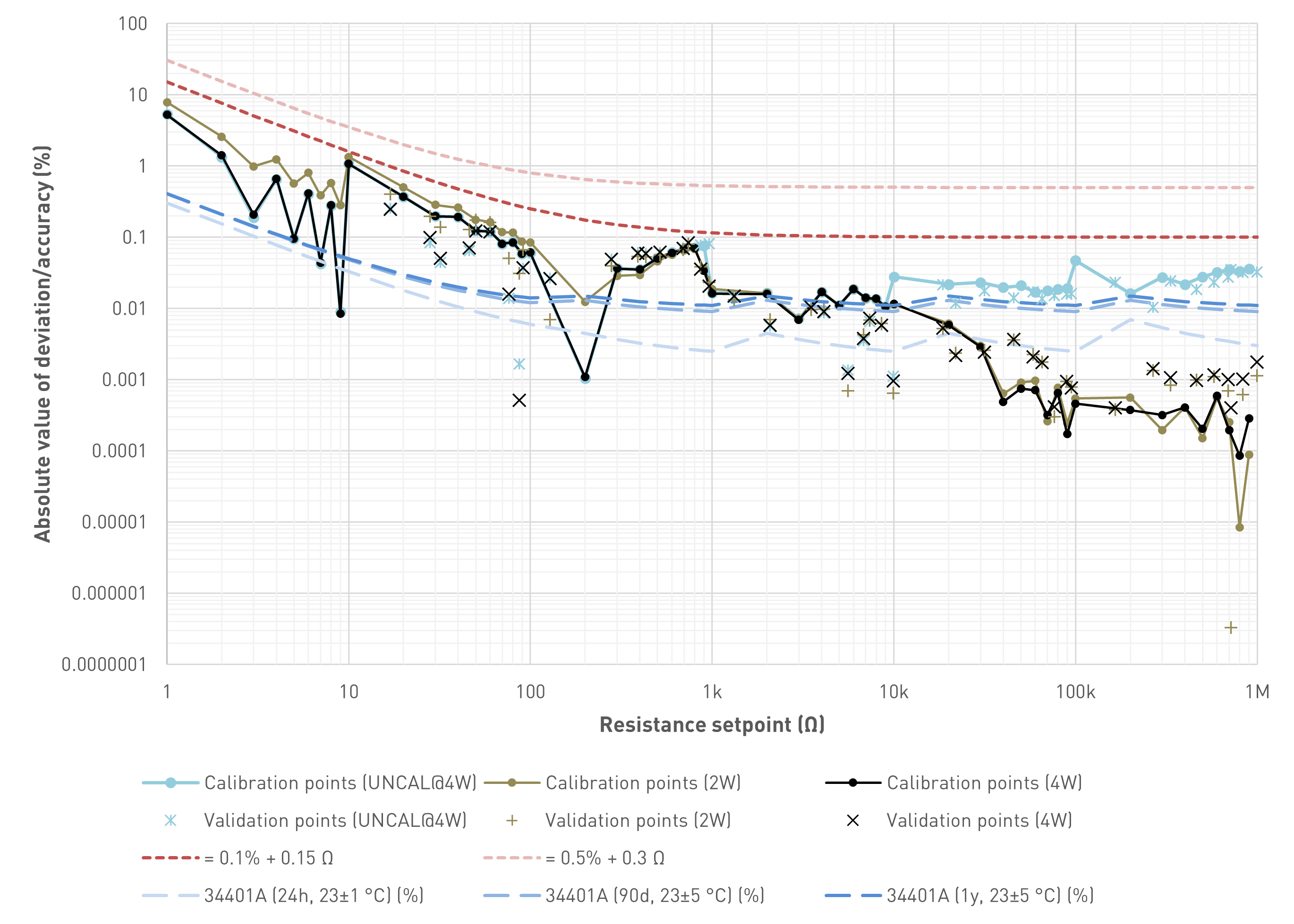
| Short-term setpoint accuracy estimate | <=±0.1% of value + 0.15 Ω (2W and 4W). The estimate is based on measurements for a limited number of calibration and validation resistance setpoints. Measurements performed with an Agilent 34401A 6.5 DMM for a single DUT. Note: This is NOT a valid strategy to get reliable/reproducible results in the sense of a specification. It's just a more or less plausible envelope based on measurements I took for my prototype. The initial goal was achieved: (much) better than ±0.5% of value + 0.3 Ω |
| Display value resolution | 6.5 digits, 5.5 digits, 4.5 digits, 3.5 digits, but not better than 1 mΩ |
| Short-term display accuracy estimate | <=±0.01% + 0.025 Ω (2W and 4W). This figure is meant to show how much the displayed resistance value (that is based on a calibration) deviates from the value shown on the DMM, the calibration has been performed with. |
| Thermal drift (estimate based on design) | <<50 ppm/K |
| Power rating | >=0.2W for decade 0 (0..9Ω), >=0.5W else Exact value depends on setpoint (shown on display) |
| Bandwidth | unspecified |
| Calibration modes | - Uncalibrated: Switches are activated according to entered setpoint, display shows setpoint - Two-wire (2W), Four-wire (4W): An internal setpoint is calculated based on the calibration values to reduce the error (effects changes for higher resistance values only) |
| Operating modes | Fixed: On trigger, no change Step: On trigger, step to trigger setpoint value Up: On trigger, increase setpoint (linearly, 1-2-3-4-5-6-7-8-9, 1-2-5, 1-3) Down: On trigger, decrease setpoint (linearly, 1-2-3-4-5-6-7-8-9, 1-2-5, 1-3) List: See list mode |
| List mode | Up to 100 values with individual dwell times - Start: on trigger; or immediately after mode selection - Step: - Auto: Advance index automatically, solely based on dwell time - Trigger: Advance index on each trigger event, ignoring the dwell time - Once: Advance index on each trigger event, only after dwell time elapsed |
| Switching | - fast (default) - break-before-make |
| Trigger | Source: Bus, External, Immediate, Manual, Timer Mode: Continuous, Single Parameter: - Delay, - Holdoff, - Slope (Rising, Falling, Either; Source: External) - Time (0.01 s .. 10^7 s; Source: Timer) |
| Inhibit | Inhibit the input - Latching: Latch input on/off on inhibit input change - Live: Switch input on/off according to present inhibit input state |
| Command and trigger execution | 10ms loops |
| User interface | - 18 digit alphanumeric display: - Primary display: Resistance setpoint - Secondary display: - Input state - max. current at setpoint - max. voltage at setpoint - max. power at setpoint - hardware setpoint - Menu-based - 6 dual color LEDs - Rotary encoder with push button - 23 additional push buttons |
| User presets | 0-9 (0 is restored on power-up) |
| Interface | - USB - Two digital inputs - settable polarity: positive, negative - function: trigger, inhibit, readout |
| Power supply | Switch mode |
Results
After the final calibration the results are in. The first diagram shows the absolute value of the deviation between the setpoint and the value indicated by the Agilent 34401A multimeter. Connecting lines between data points for visual purposes only. More details in the respective post.
Typical application
Testing software-based control loops running on embedded hardware can be very challenging. Unit and other software-only tests may catch certain errors, but will never fully cover aspects that are related to the hardware interface. The easy solution is to connect the control unit to the actual controlled process, using the sensors and actuators. However, this can be very expensive and also hard to automate. Reproducibility might suffer and in more complex cases it might be even dangerous or impossible to generate certain (error) conditions, the control unit might have to deal with.
These problems can be avoided though: We replace the controlled system including the sensors and actuators with a software simulation that interfaces with the control unit via a hardware interface: The control unit - the device under test (DUT) - is connected to a hardware-in-the-loop (HIL) simulator.
For demanding task, e. g. in the automotive world, you can buy very expensive and very capable HIL simulators that allow the operators to run highly complex simulation models of the system in real time. There are endless numbers of hardware interface options, a programmable resistor could be one of them.
For simple applications it's possible to copy this idea and implement a simple test arrangement using the programmable precision resistor. Here is an example:
The control unit (DUT) is a simple temperature controller that outputs a PWM signal used to control a fan based on the feedback provided by a thermistor (e. g. a common 10 kΩ NTC). Instead of connecting a real fan and a thermistor to the DUT, we use
- a digital multimeter to capture PWM singal's duty cycle and
- the programmable precision resistor to simulate the resistance of thermistor.
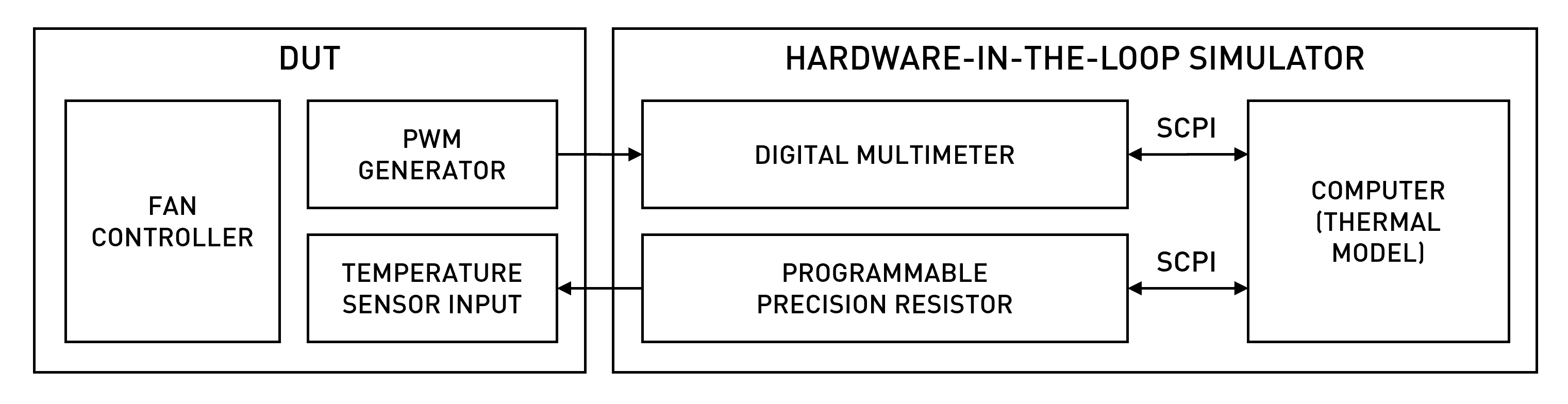
Both the digital multimeter and the programmable precision resistor are connected to a computer (communication via SCPI) that runs a thermal model of the controlled system including the fan (actuator) and the thermistor (sensor).
With this it's fairly easy to simulate
- systems with different thermal properties (robustness analysis etc.)
- different states of the controlled system: normal operation, over-temperature
- loss of signals/erroneous signals (loss of the fan PWM signal)
- malfunction of the actuator (failing fan)
- malfunction of the sensor (e. g. thermistor open, shorted)
There are multiple limitations to this setup, some of which come down to the time response:
- the SCPI-communication between the digital multimeter and the programmable precision resistor with the computer introduces delays of varying length
- the command execution loop in the programmable decade introduces delays
- relay switching introduces delays; the number of switching cycles can be of concern as well
- complexity of simulation models is limited by the computer's performance
- typical operating systems like Windows are not real-time capable (generally speaking)
In short: Use it for (very) slow systems/control loops only. Switching between different resistance values may interrupt the current flow momentarily. Depending on the DUT's input circuitry it might be possible to work around this by placing a capacitor in parallel with programmable precision resistor.
Note
All information is provided "as is" without any warranty whatsoever. Although I have compiled the information to the best of my knowledge, there might be errors. You use the information at your own risk.