After dabbling a bit with both diffusion models and VAEs, I decided to focus on CVAEs first, instead. As it seems the main problem is not the training of the network, but finding a smooth way to implement it on a MCU. So I'd rather deal with a simple architecture first to tackle the MCU implementation.

VAEs were originally introduced in 2013 in this paper. There is a very good explanation of VAEs here. 

A VAE consists of an encoder and a decoder part. The encoder is a multilayer artificial neural network (usually a CNN) that reduces the input data  to a latent representation with fewer parameters. The decoder does the opposite and expands the latent representation to a high resolution picture. The network is trained to exactly reproduce the input image on the output. In addition, there is a clever trick (the "reparamerization trick") that ensures that the latent representation is encoded in a way, where similar images are grouped. After the network is trained, we can use only the decoder part and feed in random numbers to generate new images.

Since we also want to control the number of pips on the die, we also need to label the data that is fed in - that is where the conditional part in the CVAE comes from.

The Model:Encoder

        self.encoder = nn.Sequential(
            nn.Conv2d(1 + num_classes, dim1, kernel_size=3, stride=2, padding=1),
            nn.ReLU(),
            nn.Conv2d(dim1, dim2, kernel_size=3, stride=1, padding=1),
            nn.ReLU(),
            nn.Conv2d(dim2, dim3, kernel_size=3, stride=2, padding=1),
            nn.ReLU(),
            nn.Conv2d(dim3, dim3, kernel_size=3, stride=2, padding=1),
            nn.ReLU(),
        )

        self.fc_mu = nn.Linear(dim3*4*4 + num_classes, VAE_choke_dim)
        self.fc_var = nn.Linear(dim3*4*4 + num_classes, VAE_choke_dim)

I used a simple CNN with only four layers as the encoder. The number of channels is configurable (dim1-dim3) and I will use this to investigate size/quality trade offs of the network. The dimensions are reduced from 32x32 to 4x4 in the CNN and then further to VAE_choke_dim (variable) using a fully connected network. "mu" and "var" are the expected value and the variance used in the reparameterization trick. The labels are fed into the first layer of the cnn and then again into the fully connected layer with one hot encoding. Usually one would use pooling layers and not just higher stride for dimensionality reduction, but since the encoder does not do much, this worked quite well.

The Decoder

        self.fc_decode1 = nn.Linear(VAE_choke_dim + num_classes, dim4*4*4)

        self.decoderseq = nn.Sequential(
            nn.ConvTranspose2d(dim4, dim3, kernel_size=3, stride=2, padding=1, output_padding=1),
            nn.ReLU(),
            nn.ConvTranspose2d(dim3, dim2, kernel_size=3, stride=2, padding=1, output_padding=1),
            nn.ReLU(),
            nn.ConvTranspose2d(dim2, dim1, kernel_size=3, stride=1, padding=1, output_padding=0),
            nn.ReLU(),
            nn.ConvTranspose2d(dim1, 1, kernel_size=3, stride=2, padding=1, output_padding=1),
            # nn.ReLU(),
            nn.Sigmoid()  # Remove sigmoid to simplify inference
        )

    def decoder(self, z):
        z = self.fc_decode1(z)
        z = nn.functional.relu(z)
        z = z.view(-1, dim4, 4, 4)
        return self.decoderseq(z)

The decode is basically the inverse of the encoder: a fully connected layer followed by 4 convolutional layers. The input of the decoder are the labels in one hot encoding and the latent variables that can be use to samples from the distribution.

Forward pass

    def reparameterize(self, mu, logvar):
        std = torch.exp(0.5*logvar)
        eps = torch.randn_like(std)
        return mu + eps*std * 0.5

    def forward(self, x, labels, angles):
        labels = torch.nn.functional.one_hot(labels, self.num_classes).float()
        x = torch.cat((x, labels.view(-1, self.num_classes, 1, 1).expand(-1, -1, 32, 32)), dim=1)
        h = self.encoder(x)
        h = h.view(h.shape[0], -1)
        h = torch.cat((h, labels.view(-1,self.num_classes)), dim=1)

        mu, logvar = self.fc_mu(h), self.fc_var(h)

        if VAE_reparameterize:
            z = self.reparameterize(mu, logvar)
        else:
            z = angles.unsqueeze(1).float()

        z = torch.cat((z, labels), dim=1)
        return self.decoder(z), mu, logvar

Just some plumbing here. Note that i scaled the the width of the sampling gaussian to limit the distribution of the latent variables to roughly to [-1:1]. There is an option to skip the reparametrization and instead just introduce another labels (angles). In that case, only the decoder is trained, since the encoder output is unused.

Testing and Tweaking

As a first start, I used a relatively large network with the dim parameters set to 32,32,128,128 and 10 latent variables. The network has around weights in this configuration, already requiring significant memory

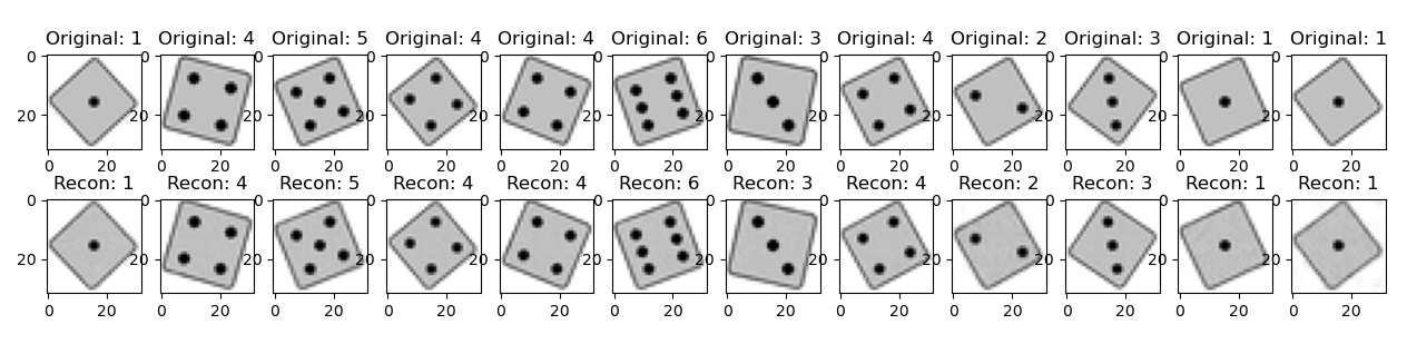
Above you can see pairs of original test images and reconstructed images from the output after training the model for 400 epochs. The reconstruction is almost pixel perfect.

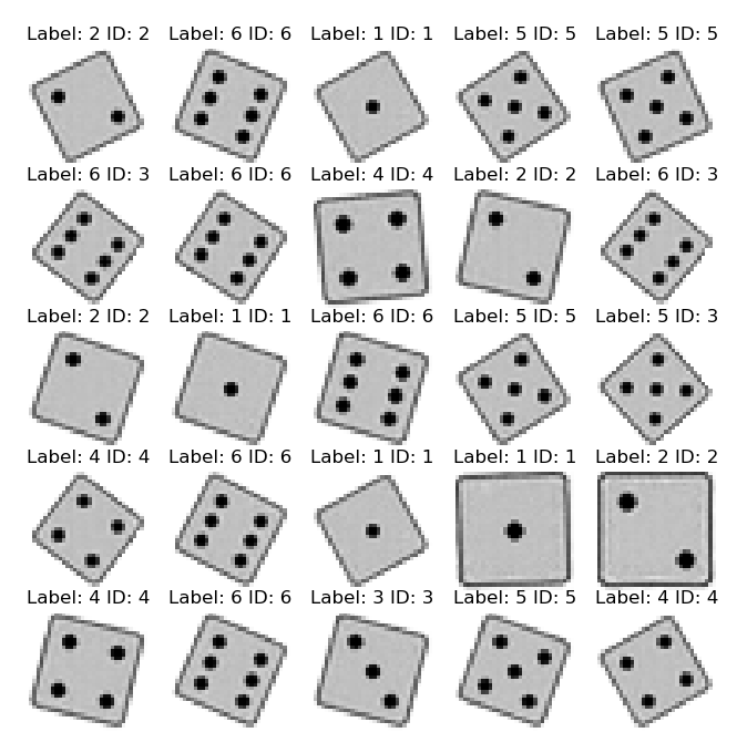
To generate images with the VAE we can feed random class labels and random latents into the decoder. The plot above shows some samples of generated images. Unfortunatley we, see many example of blurry or ghosted images now. Not all of them are properly recognized as die anymore by the evaluation CNN (see previous log), only 90.8% of 500 images were recognized properly.

The problem seems to be that I am sampling intermediate locations in the latent space. There are also not 10 variables needed to parametrize the appearance of each die, since I am basically only rotating and scaling the test images. (the class is provided as a label). One dimension is enough.

Sampling in one dimension

Changing the deminsion of the latent variable space to 1 improved generation quite a bit, with 93% passing samples. However, there were still a few outliers.

The plot above shows a scan through the entire latent variable from -1 to 1 (TL to BR) for 3 pips. We can see that the ordering is not strictly following the angle, but some other criteria. Due to this, there are a few transitional regions, where ghost images are created that look like a superposition of multiple angles instead of a smooth transition.

Simply inputting the angle as latent variable

It felt like cheating, but I resorted to simply inputting the angle of the die as a variable. This ensures that the varible is learned in a sensible order. Since the encoder is bypassed, only the decoder is trained. Stricty speaking, we do not have a VAE anymore. However, since I already have the architecture in place I could use it for other training sets later than do not have to rely on such a strict ordering. (There are also better ways of sampling by relying on the learned distribution - but i wanted to keep it simepl).

The plot above shows samples if images generated with the trained decoder. The accuracy with the evaluation network is now 100%. (500/500).

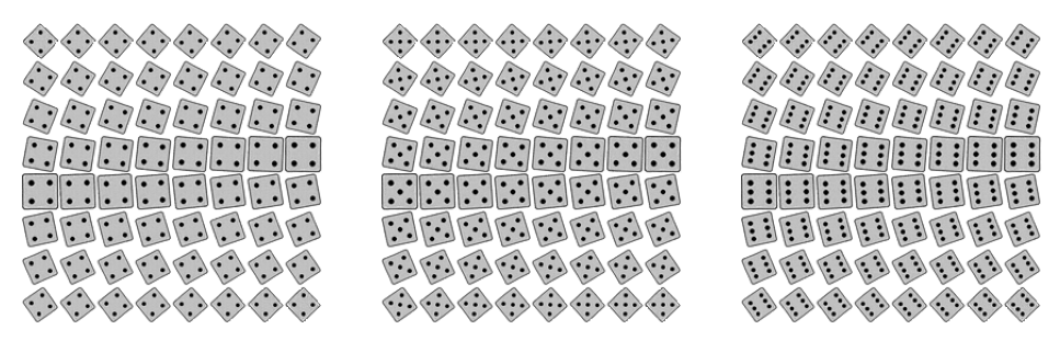
A latent space scan for the classes 4,5,6 is shown above. As expected, the rotation of the dies is encoded in order now.