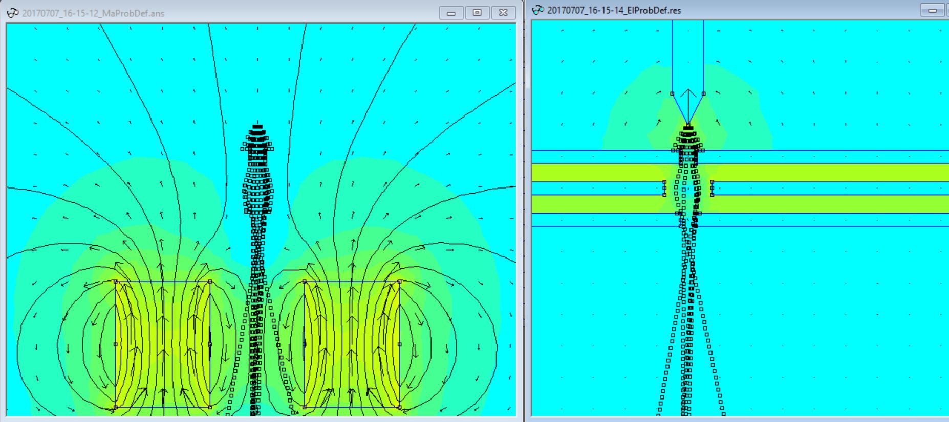
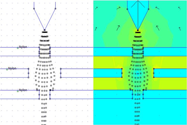
In last month I optimized how both parts of the simulation (electrical, magnetical) interact. But it is still one major piece of the simulation missing. May you can see it on the top left image. The particles are not response to the magnetic field. But the particles response to the electrical field, what you see on the top left image. One the left image you see a tip with -100 volt and the trace of the electrons. The particles are accelerated by the electrical field between the tip and the first plate. The first plate has a voltage of 0 volt. The plate in the middle has again -100 volt and the last one has again 0 volt. The voltage differences are the reason why the electron traces are bented. At the first plate at the edges you can see that if a electron touch a object it stops. The electrons cross both parts of the simulation the electrical and the magnetical. Therefore you see the traces on the left and the right side of the image

The current version I uploaded on Github. to run the simulation you need the FEMM 4.2. In the folder where the DIY-SEM-G04 is located you have to create two folder. Probdef for the simulation and SimPictures for the storage of the images. Without these folders you get a error.

to run the simulation open FEMM 4.2 click on the button, select the file and that it. Now the Simulation need some minutes and after that you find the images in the SimPictures folder.

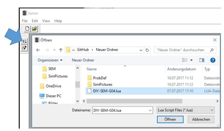
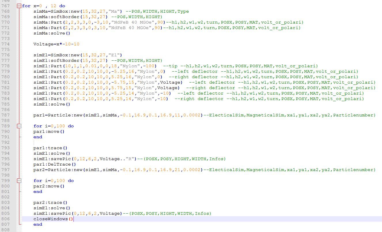
For writing the code I use Notepad++. Lets do a quick walk through the code. At the beginning a SimBox needs to create. With the "Ma" is a magnetical and with a "El" is a electrical simulation box created. As next a softBorder needs to create.

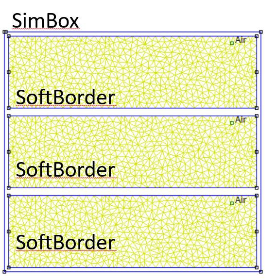
The concept of the soft borders is that this give you the opportunity to separate part from each other. The particles can cross the soft borders but not the SimBox. If a particle touch the SimBox it stops. In the example code the size of the SimBox and the Softborder is equal therefore it appear only one box.

With the lines ... :Part(...) the objects are placed.

All objects are base on a pentagon. The parameters are

• H1 H2: Height
• W1 W2: Wide
• Turn: rotation in grade about the cente
• Posx Posy: Postion of the center
• Mat: Material of the object
• Volt or Polari: Voltage if the object is in a electrical simulation or the polarity in grade of the magnet if the object is in a magnetical simulation

With the lines ... :solve() are the magnetic and electrical fields are calculated. Afterwards the start point of the particles is defined with the line Particle:new(Sim,Sim,x1,y1,x2,y2,amount,step). The variable Sim contains which fields shall apply to the particles. The variables x,1y1,x2,y2 are the start and end points of a line on which the particles are placed. The variable amount is number of particles which are placed . The variable step contains the information what is the expect step size for the particle (It is the parameter S). The unit is in meter therefore is a step size of 0.2mm = 0.0002 m.

With the function ... :move() calculates the next positions of the particle. This function is repeatedly because with each call is a distance of the size step calculated. In the example it is called 100 times therefore the particles can travel 20mm=100*0.2mm.

The function ... :trace() bring the traces of the particles in the simulation see on the left side. To get a nice colorfully image the ... :solve() function has to called again.

if the the ...:trace(1) is called instead of trace() then the points will be connected with blue lines. But careful if the traces of participles cross each other then no image can be created.

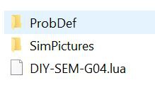
With the line ... :savePic(...) is a image stored in the folder "SimPictures". The Parameter of the savePic function are the following:

• POSX,POSY: the center of the image
• HEIGHT: the height of the image
  • (if the value is to small the image looks strange)
• WIDTH: the width of the image
  • (if the value is to small the image looks strange)
• Infos: a sting shown in the file name of the image

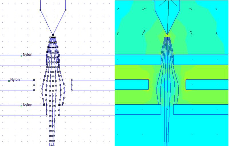
Above you can see the mesh for the field calculation. As finer the gird as preciser field calculation. To get a finer grid two groups of particles are used. The first group par1 moved through the field and creates traces. The rough field is shown on the left side. With the traces the field is calculated again. This fine field is shown on the right side. To just see the second group (par2) of particles the first group (par1) is removed with the function ... :DelTraces. After that the second group of paricles (par2) is created and moved through the field the windows are closed with the line closeWindows().

The animation above show the trace of a rough mesh and a voltage change -10V to -130of the middle plate.

The animation above show the trace of a fine mesh and a voltage change from -10V to -130Vof the middle plate.