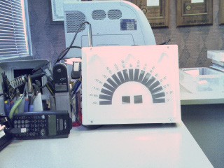
A popular way of presenting polarization information is by recognizing that the three main polarization components – polarization intensity, Degree of Linear Polarization, and Angle of Polarization - are analogous to the color components of brightness, saturation, and hue. The HSV (Hue, Saturation, Value) model provides better contrast and more quantifiable information about a scene’s polarization than the simple RGB merge that I have been using so far. Here are the "normal" and RGB polarization images for my test target:

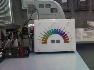
In contrast, the HSV representation really hones in on polarized light:

WOW!!!! Everything that is not linearly polarized just went completely dark, while polarized light on the other hand really pops out!!! Can you spot the LCDs on my calculator and digital calipers? Also notice the perfect encoding of linear angle of polarization (AoP) by color.

It's remarkable that there is no back-illumination involved whatsoever. The three images above were acquired by DOLPi-MECH under identical conditions on my workbench. Illumination comes solely from overhead fluorescent lights and some late-afternoon sunlight seeping through the window blinds.

The Python code to render the HSV image is:

    #convert images to signed double (int16)
    image0_d=np.int16(image0)
    image90_d=np.int16(image90)
    image45_d=np.int16(image45)
    image135_d=np.int16(image135)
    imageLHCP_d=np.int16(imageLHCP)
    imageRHCP_d=np.int16(imageRHCP)
    #calculate Stokes parameters
    stokesI=image0_d+image90_d+1
    stokesQ=image0_d-image90_d
    stokesU=image45_d-image135_d
    stokesV=imageLHCP_d-imageRHCP_d
    #calculate polarization parameters
    polInt=np.sqrt(1+np.square(stokesQ)+np.square(stokesU))  #Linear Polarization Intensity
    polDoLP=polInt/stokesI   #Degree of Linear Polarization
    polAoP=0.5*(np.arctan2(stokesU,stokesQ))  #Angle of Polarization
    polDoCP=(2*np.absolute(stokesV))/polInt  #Degree of Circular Polarization

    #prepare DOLPi HSV image
    H=np.uint8((polAoP+(3.1416/2))*(180/3.1416))
    S=np.uint8(255*(polDoLP/np.amax(polDoLP)))
    V=np.uint8(255*(polInt/np.amax(polInt)))

    imageDOLPiHSV=cv2.merge([H,S,V])
    DOLPiHSVinBGR=cv2.cvtColor(imageDOLPiHSV,cv2.COLOR_HSV2BGR)
    cv2.imshow("DOLPi_HSV",DOLPiHSVinBGR)

You may notice that OpenCV (cv2) assumes the following ranges for the HSV parameters:

Hue = H = 0 to 180 (please refer to the main project's white paper for an explanation)

Saturation = S = 0 to 255

Value (Intensity) = V = 0 to 255

The HSV tuple is then converted into a BGR tuple that can be displayed through cv2.imshow (cv2 uses BGR instead of RGB encoding for color images).

Next - I'll work on integrating the polarization analysis and real-time HSV into the electro-optic DOLPi's code and compare its performance against that of the much slower but more precise DOLPI-MECH.

Here is the complete code as it currently stands for DOLPi-MECH:

#   DOLPiMech2.py
#
#   This Python program demonstrates the DOLPi_Mech polarimetric camera.
#
#   A servo motor rotates a polarization filter wheel in front of the
#   Raspberry Pi camera.  An Adafruit PWM Servo HAT drives the servo.
#
#   (c) 2015 David Prutchi, Ph.D., licensed under MIT license
#                                  (MIT, opensource.org/licenses/MIT)
#
#
#import the necessary packages
from picamera.array import PiRGBArray
from picamera import PiCamera
import time
import cv2
from Adafruit_PWM_Servo_Driver import PWM
import numpy as np
import matplotlib.pyplot as plt

def dispStokes(stokesI, stokesQ, stokesU, stokesV):
    #Function dispStokes - Save and optionally display Stokes parameters
    plt.figure("Stokes")
    plt.subplot(2,2,1)
    plt.imshow(stokesI)
    plt.axis('off')
    plt.title("Stokes I")
    #
    plt.subplot(2,2,2)
    plt.imshow(stokesQ)
    plt.axis('off')
    plt.title("Stokes Q")
    #
    plt.subplot(2,2,3)
    plt.imshow(stokesU)
    plt.axis('off')
    plt.title("Stokes U")
    #
    plt.subplot(2,2,4)
    plt.imshow(stokesV)
    plt.axis('off')
    plt.title("Stokes V")
    #
    plt.savefig('Stokes.png',bbox_inches='tight')
    plt.show(block=False)

def dispPol(polInt, polDoLP, polAoP, polDoCP):   
    #Function dispPol - Save and optionally display polarization parameters
    plt.figure("pol")
    plt.subplot(2,2,1)
    plt.imshow(polInt)
    plt.axis('off')
    plt.title("Linear Pol Intensity")
    #
    plt.subplot(2,2,2)
    plt.imshow(polDoLP)
    plt.axis('off')
    plt.title("DoLP")
    #
    plt.subplot(2,2,3)
    plt.imshow(polAoP)
    plt.axis('off')
    plt.title("AoP")
    #
    plt.subplot(2,2,4)
    plt.imshow(polDoCP)
    plt.axis('off')
    plt.title("DoCP")
    #
    plt.savefig('polarization.png',bbox_inches='tight')
    plt.show(block=False)

# Initialise the Adafruit PWM HAT using the default address
pwm = PWM(0x40)
pwm.setPWMFreq(60)   # Set PWM frequency to 60 Hz
servoMin = 180       # Min pulse length out of 4096
servoMax = 615       # Max pulse length out of 4096
# Servo PWM values for different filter wheel positions
servoNone = 615      # PWM setting for open window
servo0=541           # PWM setting for 0 degree filter
servo90=468          # PWM setting for 90 degree filter
servo45=395          # PWM setting for 45 degree filter
servo135=321         # PWM setting for -45 degree (=135 degree) filter
servoLHCP=247        # PWM setting for LHCP filter
servoRHCP=180        # PWM setting for RHCP filter

#Raspberry Pi Camera Initialization
#----------------------------------
#Initialize the camera and grab a reference to the raw camera capture
camera = PiCamera()
camera.resolution = (320, 240)
#camera.resolution = (640, 480)
#camera.resolution = (1280,720)
camera.framerate=30
rawCapture = PiRGBArray(camera)
camera.led=False

#Auto-Exposure Lock
#------------------
# Wait for the automatic gain control to settle
time.sleep(2)
# Now fix the values
camera.shutter_speed = camera.exposure_speed
camera.exposure_mode = 'off'
gain = camera.awb_gains
camera.awb_mode = 'off'
camera.awb_gains = gain

#Initialize flags
loop=True  #Initial state of loop flag
first=False #Flag to skip display during first loop
video=False #Use video port?  Video is faster, but image quality is significantly
            #lower than using still-image capture

while loop:
    #grab an image from the camera with no filter
    pwm.setPWM(0, 0, servoNone)
    time.sleep(0.5)
    rawCapture.truncate(0)
    camera.capture(rawCapture, format="bgr",use_video_port=video)
    imageNone=rawCapture.array

    #grab an image from the camera with linear polarizer at 0 degrees
    pwm.setPWM(0, 0, servo0)
    time.sleep(0.1)    #Wait for filter wheel to move
    rawCapture.truncate(0)
    camera.capture(rawCapture, format="bgr",use_video_port=video)
    image0=cv2.cvtColor(rawCapture.array,cv2.COLOR_BGR2GRAY)
    
    #grab an image from the camera with linear polarizer at 90 degrees
    pwm.setPWM(0, 0, servo90)
    time.sleep(0.1)
    rawCapture.truncate(0)
    camera.capture(rawCapture, format="bgr",use_video_port=video)
    image90=cv2.cvtColor(rawCapture.array,cv2.COLOR_BGR2GRAY)

    #grab an image from the camera with linear polarizer at 45 degrees
    pwm.setPWM(0, 0, servo45)
    time.sleep(0.1)
    rawCapture.truncate(0)
    camera.capture(rawCapture, format="bgr",use_video_port=video)
    image45=cv2.cvtColor(rawCapture.array,cv2.COLOR_BGR2GRAY)

    #grab an image from the camera with linear polarizer at -45 degrees (=135 degrees)
    pwm.setPWM(0, 0, servo135)
    time.sleep(0.1)
    rawCapture.truncate(0)
    camera.capture(rawCapture, format="bgr",use_video_port=video)
    image135=cv2.cvtColor(rawCapture.array,cv2.COLOR_BGR2GRAY)

    #grab an image from the camera with LHCP filter
    pwm.setPWM(0, 0, servoLHCP)
    time.sleep(0.1)
    rawCapture.truncate(0)
    camera.capture(rawCapture, format="bgr",use_video_port=video)
    imageLHCP=cv2.cvtColor(rawCapture.array,cv2.COLOR_BGR2GRAY)

    #grab an image from the camera with RHCP filter
    pwm.setPWM(0, 0, servoRHCP)
    time.sleep(0.1)
    rawCapture.truncate(0)
    camera.capture(rawCapture, format="bgr",use_video_port=video)
    imageRHCP=cv2.cvtColor(rawCapture.array,cv2.COLOR_BGR2GRAY)
    
    #convert images to signed double (int16)
    image0_d=np.int16(image0)
    image90_d=np.int16(image90)
    image45_d=np.int16(image45)
    image135_d=np.int16(image135)
    imageLHCP_d=np.int16(imageLHCP)
    imageRHCP_d=np.int16(imageRHCP)
    #calculate Stokes parameters
    stokesI=image0_d+image90_d+1
    stokesQ=image0_d-image90_d
    stokesU=image45_d-image135_d
    stokesV=imageLHCP_d-imageRHCP_d
    #calculate polarization parameters
    polInt=np.sqrt(1+np.square(stokesQ)+np.square(stokesU))  #Linear Polarization Intensity
    polDoLP=polInt/stokesI   #Degree of Linear Polarization
    polAoP=0.5*(np.arctan2(stokesU,stokesQ))  #Angle of Polarization
    polDoCP=(2*np.absolute(stokesV))/polInt  #Degree of Circular Polarization

    #prepare DOLPi HSV image
    H=np.uint8((polAoP+(3.1416/2))*(180/3.1416))
    S=np.uint8(255*(polDoLP/np.amax(polDoLP)))
    V=np.uint8(255*(polInt/np.amax(polInt)))

    #The following block is just for debugging
    #-----------------------------------------
    #plt.imshow(H)
    #plt.axis('off')
    #plt.title("H=AoP")
    #plt.colorbar()
    #plt.show()
    #
    #plt.imshow(S)
    #plt.axis('off')
    #plt.title("S=polDoLP")
    #plt.colorbar()
    #plt.show()
    #
    #plt.imshow(V)
    #plt.axis('off')
    #plt.title("V=polInt")
    #plt.colorbar()
    #plt.show()

    #prepare DOLPi RGB image
    R=image0
    B=image90
    G=image45
    imageDOLPi=cv2.merge([B,G,R])
    cv2.imshow("Image_DOLPi",imageDOLPi)  #Display DOLPi preview image


    imageDOLPiHSV=cv2.merge([H,S,V])
    DOLPiHSVinBGR=cv2.cvtColor(imageDOLPiHSV,cv2.COLOR_HSV2BGR)
    cv2.imshow("DOLPi_HSV",DOLPiHSVinBGR)
     
    
    #cv2.imshow("Image_DOLPi",cv2.resize(imageDOLPi,(320,240),interpolation=cv2.INTER_AREA))  #Display DOLP image
    k = cv2.waitKey(1)  #Check keyboard for input
    if k == ord('x'):   # wait for x key to exit
        loop=False
    

#   Save and Prepare to leave
#   -------------------------
#
pwm.setPWM(0, 0, servoNone) #return filter wheel to no-filter position
#display and save calculated polarization parameters
dispStokes(stokesI, stokesQ, stokesU, stokesV)
dispPol(polInt, polDoLP, polAoP, polDoCP)


#save images
cv2.imwrite("imageNone.jpg",imageNone)
cv2.imwrite("image0.jpg",image0)
cv2.imwrite("image90.jpg",image90)
cv2.imwrite("image45.jpg",image45)
cv2.imwrite("image135.jpg",image135)
cv2.imwrite("imageLHCP.jpg",imageLHCP)
cv2.imwrite("imageRHCP.jpg",imageRHCP)
cv2.imwrite("RGBpol.jpg",cv2.merge([B,G,R]))
cv2.imwrite("HSVpol.jpg",DOLPiHSVinBGR)
#exit
time.sleep(10)
cv2.destroyAllWindows()
quit