Fitting a Quadratic Bezier Curve to Point Data

Fitting a Quadratice Bezier Curve to Digitised Data

Here is the problem image:

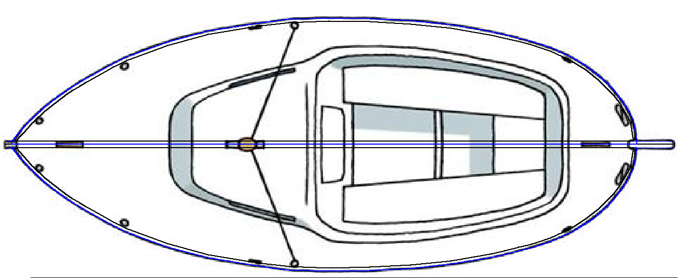
(source: https://www.oostzeejol.de/index.php/en/international-2/lynaes-14)

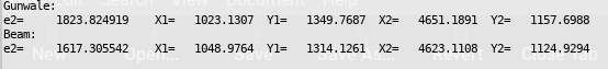
The blue and black digitised lines are the Gunwale and Sheer (beam) of the sailboat design I want to reverse engineer. The image is a plan of the Lynaes 14 sailboat that I found on the Internet.

I have previously tried to model the beam in Excel using polynomial curve fitting but the results were not satisfactory.

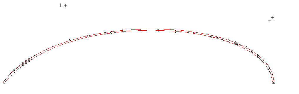
However, fitting quadratic Bezier curves was excellent:

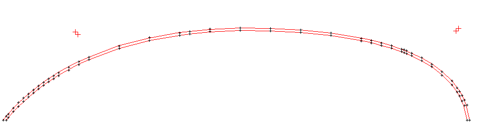
The image has four Bezier curves joined at the max beam.

Note how well the Bezier curves meet at the stern. This is a problem area for polynomial curves.

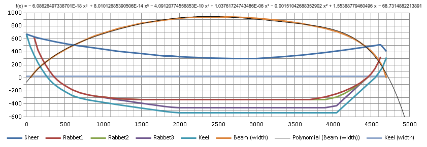
Here is the polynomial 6th order fit. While it looks okay at this scale, the beam wanders and the curve at the stern is not ideal (i.e. perpendicular):

Here is an image of a Lynaes 14 stern which is near perpendular to the keel:

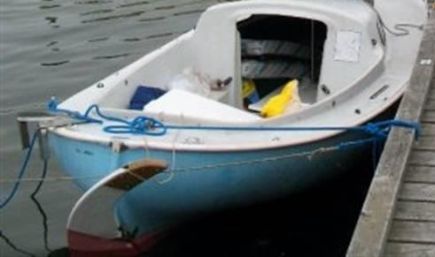
(source: https://www.baadgalleri.dk/galleri/billeder/lynaes-14/5243)

Project Logs

Collapse

Code for Cubic Bezier Version

agp.cooper • 02/18/2024 at 11:00 • 0 comments

Cubic Code Results

While the results are good it is not exact like the piece-wise quadratic bezier code.

I quess a fourth order bezier would bit better.

Hers is the cubic match:

Note the bezier cuves are too wide just aft of the maxium beam and too narrow near the stern.

Here are the control points:

Here is the full code:

// Include libraries
#include <stdio.h>
#include <stdlib.h>
#include <stdbool.h>
#include <string.h>
#include <math.h>

// Include in local directory:
#include "ezxdisp.h"
// Library: libezx.a 
// Linker: -L. -lezx -lX11 -lm

// EZX window size
static int width=1200;
static int height=700;
static double scale=0.2;
// EZX display
static ezx_t *disp;

void PlotBezier(double Xi[],double Yi[],double Ti[],int Ni,double *Bx1,double *By1,double *Bx2,double *By2)
{
  // Plot Fitted Bezier Curve  
  double X0,Y0,X1,Y1;
  X1=Xi[0];
  Y1=Yi[0];
  for (int i=1;i<Ni;i++) {
	double t=1.0*i/(Ni-1);
  	double s=(1.0-t);
	X0=X1;
	Y0=Y1;
    X1=s*s*s*Xi[0]+3*s*s*t**Bx1+3*s*t*t**Bx2+t*t*t*Xi[Ni-1];
    Y1=s*s*s*Yi[0]+3*s*s*t**By1+3*s*t*t**By2+t*t*t*Yi[Ni-1];
    ezx_line_2d(disp,scale*X0,height/2-scale*Y0,scale*X1,height/2-scale*Y1,&ezx_red,1);
  }
  
  // Plot Fitted Control Point (B1)
  ezx_line_2d(disp,scale**Bx1-5,height/2-scale**By1,scale**Bx1+5,height/2-scale**By1,&ezx_black,1);
  ezx_line_2d(disp,scale**Bx1,height/2-scale**By1-5,scale**Bx1,height/2-scale**By1+5,&ezx_black,1);

  // Plot Fitted Control Point (B2)
  ezx_line_2d(disp,scale**Bx2-5,height/2-scale**By2,scale**Bx2+5,height/2-scale**By2,&ezx_black,1);
  ezx_line_2d(disp,scale**Bx2,height/2-scale**By2-5,scale**Bx2,height/2-scale**By2+5,&ezx_black,1);
  
  // Plot Input points     
  for (int i=0;i<Ni;i++) {
    ezx_line_2d(disp,scale*Xi[i]-2,height/2-scale*Yi[i]-2,scale*Xi[i]+2,height/2-scale*Yi[i]+2,&ezx_black,1);
    ezx_line_2d(disp,scale*Xi[i]+2,height/2-scale*Yi[i]-2,scale*Xi[i]-2,height/2-scale*Yi[i]+2,&ezx_black,1);
  }
  
  return;
}


void FitBezier(double Xi[],double Yi[],double Ti[],int Ni,double *x1,double *y1,double *x2,double *y2)
{
  double Bx0=Xi[0];
  double By0=Yi[0];
  double Bx1=*x1;
  double By1=*y1;
  double Bx2=*x2;
  double By2=*y2;
  double Bx3=Xi[Ni-1];
  double By3=Yi[Ni-1];
  double Ex1,E1x1,E2x1;
  double Ey1,E1y1,E2y1;
  double Ex2,E1x2,E2x2;
  double Ey2,E1y2,E2y2;
  double t,e2=0.0;
  do {
    E1x1=0.0;
    E2x1=0.0;
    E1y1=0.0;
    E2y1=0.0;
    E1x2=0.0;
    E2x2=0.0;
    E1y2=0.0;
    E2y2=0.0;
    e2=0.0;
    // Solve all t
    for (int i=1;i<Ni-1;i++) {

      double Et=0.0;
      t=Ti[i]; // Initial t
      // printf("i=%3d t=%12.6lf",i,t);
      do {
        double f1=(t*t*t*(-Bx0+3*Bx1-3*Bx2+Bx3)+t*t*(3*Bx0-6*Bx1+3*Bx2)+t*(-3*Bx0+3*Bx1)+(Bx0-Xi[i]))*(6*t*t*(-Bx0+3*Bx1-3*Bx2+Bx3)+4*t*(3*Bx0-6*Bx1+3*Bx2)+2*(-3*Bx0+3*Bx1))
                 +(t*t*t*(-By0+3*By1-3*By2+By3)+t*t*(3*By0-6*By1+3*By2)+t*(-3*By0+3*By1)+(By0-Yi[i]))*(6*t*t*(-By0+3*By1-3*By2+By3)+4*t*(3*By0-6*By1+3*By2)+2*(-3*By0+3*By1));
        double f2=(3*t*t*(-Bx0+3*Bx1-3*Bx2+Bx3)+2*t*(3*Bx0-6*Bx1+3*Bx2)+(-3*Bx0+3*Bx1))*(6*t*t*(-Bx0+3*Bx1-3*Bx2+Bx3)+4*t*(3*Bx0-6*Bx1+3*Bx2)+2*(-3*Bx0+3*Bx1))
                 +(t*t*t*(-Bx0+3*Bx1-3*Bx2+Bx3)+t*t*(3*Bx0-6*Bx1+3*Bx2)+t*(-3*Bx0+3*Bx1)+(Bx0-Xi[i]))*(12*t*(-Bx0+3*Bx1-3*Bx2+Bx3)+4*(3*Bx0-6*Bx1+3*Bx2))
                 +(3*t*t*(-By0+3*By1-3*By2+By3)+2*t*(3*By0-6*By1+3*By2)+(-3*By0+3*By1))*(6*t*t*(-By0+3*By1-3*By2+By3)+4*t*(3*By0-6*By1+3*By2)+2*(-3*By0+3*By1))
                 +(t*t*t*(-By0+3*By1-3*By2+By3)+t*t*(3*By0-6*By1+3*By2)+t*(-3*By0+3*By1)+(By0-Yi[i]))*(12*t*(-By0+3*By1-3*By2+By3)+4*(3*By0-6*By1+3*By2));
        Et=f1/f2;
        t=t-Et;
      } while (Et*Et>1e-8); // Error ~0.001      
      Ti[i]=t;
      e2=e2+(Bx0*(1-t)*(1-t)*(1-t)+3*Bx1*(1-t)*(1-t)*t+3*Bx2*(1-t)*t*t+Bx3*t*t*t-Xi[i])*(Bx0*(1-t)*(1-t)*(1-t)+3*Bx1*(1-t)*(1-t)*t+3*Bx2*(1-t)*t*t+Bx3*t*t*t-Xi[i])
           +(By0*(1-t)*(1-t)*(1-t)+3*By1*(1-t)*(1-t)*t+3*By2*(1-t)*t*t+By3*t*t*t-Yi[i])*(By0*(1-t)*(1-t)*(1-t)+3*By1*(1-t)*(1-t)*t+3*By2*(1-t)*t*t+By3*t*t*t-Yi[i]);
      // printf(" -> t=%12.6lf Et*Et=%12.6lf",t,Et*Et);getchar();

      // WRT: Bx1
      E1x1=E1x1+6*t*(t*t*t*(-Bx0+3*Bx1-3*Bx2+Bx3)+t*t*(3*Bx0-6*Bx1+3*Bx2)+t*(-3*Bx0+3*Bx1)+(Bx0-Xi[i]))*(t*t-2*t+1);
      E2x1=E2x1+18*t*t*(t*t-2*t+1)*(t*t-2...

New and Improved Version
agp.cooper • 02/12/2024 at 02:11 • 0 comments
Code Rebuild
I rebuilt the code for a different staing point. Instead of:
B(t)=(1-t)^2*B0+2*t*(1-t)*B1+t^2*B2
I refacted the equation to:
B(t)=(B0-2*B1+B2)*t^2+2*(B1-B0)*t+B0
The error squared for each "t" is:
e^2=((Bx0-2*Bx1+Bx2)*t^2+2*(Bx1-Bx0)*t+Bx0-Xi)^2
+((By0-2*By1+By2)*t^2+2*(By1-By0)*t+By0-Yi)^2
This equation (e2) calculates the square of distance between the interpolated point (Xi,Yi) from the closest point on the "trial" Bezier curve.
The updated procedure is:
```
void FitBezier(double Xi[],double Yi[],double Ti[],int Ni,double *x1,double *y1)
{
  double Bx0=Xi[0];
  double By0=Yi[0];
  double Bx1=*x1;
  double By1=*y1;
  double Bx2=Xi[Ni-1];
  double By2=Yi[Ni-1];
  double Ex,E1x1,E2x1;
  double Ey,E1y1,E2y1;
  double t;
  do {
    E1x1=0.0;
    E2x1=0.0;
    E1y1=0.0;
    E2y1=0.0;
    // Solve all t
    for (int i=1;i<Ni-1;i++) {
      // Solve t
      double b4=(Bx0-2*Bx1+Bx2)*(Bx0-2*Bx1+Bx2)+(By0-2*By1+By2)*(By0-2*By1+By2);
      double b3=(Bx0-2*Bx1+Bx2)*(Bx1-Bx0)+(By0-2*By1+By2)*(By1-By0);
      double b2=2*(Bx1-Bx0)*(Bx1-Bx0)+(Bx0-2*Bx1+Bx2)*(Bx0-Xi[i])+2*(By1-By0)*(By1-By0)+(By0-2*By1+By2)*(By0-Yi[i]);
      double b1=(Bx1-Bx0)*(Bx0-Xi[i])+(By1-By0)*(By0-Yi[i]);
      // double b0=(Bx0-Xi[i])*(Bx0-Xi[i])+(By0-Yi[i])*(By0-Yi[i]);
      double Et=0.0;
      t=Ti[i]; // Initial t
      do {
        double Et1=4*t*t*t*b4+12*t*t*b3+4*t*b2+4*b1;
        double Et2=12*t*t*b4+24*t*b3+4*b2;
        Et=Et1/Et2;
        t=t-Et;
      } while (Et*Et>1e-6); // Error ~0.001      
      Ti[i]=t;
      E1x1=E1x1+(-4*(Bx0-2*Bx1+Bx2))*t*t*t*t+4*(-2*(Bx1-Bx0)+(Bx0-2*Bx1+Bx2))*t*t*t+4*(2*(Bx1-Bx0)-(Bx0-Xi[i]))*t*t+4*(Bx0-Xi[i])*t;
      E2x1=E2x1+8*t*t*t*t-16*t*t*t+8*t*t;
      E1y1=E1y1+(-4*(By0-2*By1+By2))*t*t*t*t+4*(-2*(By1-By0)+(By0-2*By1+By2))*t*t*t+4*(2*(By1-By0)-(By0-Yi[i]))*t*t+4*(By0-Yi[i])*t;
      E2y1=E2y1+8*t*t*t*t-16*t*t*t+8*t*t;
    }
    Ex=E1x1/E2x1;
    Ey=E1y1/E2y1;   
    Bx1=Bx1-Ex;
    By1=By1-Ey;    
  } while (Ex*Ex+Ey*Ey>1e-6); // Error ~0.001
  *x1=Bx1;
  *y1=By1;
  
  return;
}
```
Derivation
Only interesting if you want to do it yourself!
Refactorise B(t):
B(t)=(1-t)^2*B0+2*t*(1-t)*B1+t^2*B2
=(B0-2*B1+B2)*t^2+2*(B1-B0)*t+B0

Solve Derivatives for e2 with respect to "t":
e2=((Bx0-2*Bx1+Bx2)*t^2+2*(Bx1-Bx0)*t+Bx0-Xi)^2+((By0-2*By1+By2)*t^2+2*(By1-By0)*t+By0-Yi)^2
=((Bx0-2*Bx1+Bx2)*t^2+2*(Bx1-Bx0)*t+Bx0-Xi)^2
+((By0-2*By1+By2)*t^2+2*(By1-By0)*t+By0-Yi)^2
=(Bx0-2*Bx1+Bx2)*(Bx0-2*Bx1+Bx2)*t^4
+4*(Bx1-Bx0)*(Bx1-Bx0)*t^2
+ (Bx0-Xi)*(Bx0-Xi)
+2*(Bx0-2*Bx1+Bx2)*t^2*2*(Bx1-Bx0)*t
+2*(Bx0-2*Bx1+Bx2)*t^2 *(Bx0-Xi)
+2*2*(Bx1-Bx0)*t*(Bx0-Xi)
+...
=t^4 *(Bx0-2*Bx1+Bx2)*(Bx0-2*Bx1+Bx2)
+t^2*4*(Bx1-Bx0)*(Bx1-Bx0)
+ (Bx0-Xi)*(Bx0-Xi)
+t^3*4*(Bx0-2*Bx1+Bx2)*(Bx1-Bx0)
+t^2*2*(Bx0-2*Bx1+Bx2)*(Bx0-Xi)
+t *4*(Bx1-Bx0)*(Bx0-Xi)
+...
=t^4 *(Bx0-2*Bx1+Bx2)*(Bx0-2*Bx1+Bx2)
+t^3*4*(Bx0-2*Bx1+Bx2)*(Bx1-Bx0)
+t^2*2*(2*(Bx1-Bx0)*(Bx1-Bx0)+(Bx0-2*Bx1+Bx2)*(Bx0-Xi))
+t *4*(Bx1-Bx0)*(Bx0-Xi)
+ (Bx0-Xi)*(Bx0-Xi)
+...
=t^4 *(Bx0-2*Bx1+Bx2)*(Bx0-2*Bx1+Bx2)
+t^3*4*(Bx0-2*Bx1+Bx2)*(Bx1-Bx0)
+t^2*2*(2*(Bx1-Bx0)*(Bx1-Bx0)+(Bx0-2*Bx1+Bx2)*(Bx0-Xi))
+t *4*(Bx1-Bx0)*(Bx0-Xi)
+ (Bx0-Xi)*(Bx0-Xi)
+t^4 *(By0-2*By1+By2)*(By0-2*By1+By2)
+t^3*4*(By0-2*By1+By2)*(By1-By0)
+t^2*2*(2*(By1-By0)*(By1-By0)+(By0-2*By1+By2)*(By0-Yi))
+t *4*(By1-By0)*(By0-Yi)
+ (By0-Yi)*(By0-Yi)

=t^4 *((Bx0-2*Bx1+Bx2)*(Bx0-2*Bx1+Bx2)+(By0-2*By1+By2)*(By0-2*By1+By2))
+t^3*4*((Bx0-2*Bx1+Bx2)*(Bx1-Bx0)+(By0-2*By1+By2)*(By1-By0))
+t^2*2*(2*(Bx1-Bx0)*(Bx1-Bx0)+(Bx0-2*Bx1+Bx2)*(Bx0-Xi)+2*(By1-By0)*(By1-By0)+(By0-2*By1+By2)*(By0-Yi))...
Read more »
A Non-Suleiman IP Version
agp.cooper • 01/31/2024 at 13:32 • 0 comments

Non-Suleiman Version
After my last post I realised I did not need Suleiman's code. The Newton-Rapson method could solve the "t" values directly, but it would likely need more iterations.
Here are the results:
So the results are indentical which means my derivation (based on first and second derivates) is but a refactorisation of Suleiman's.
BezierFitV2.c is in the files directory.
Coding a Solution
agp.cooper • 01/31/2024 at 07:49 • 0 comments

Mapping Digitised Points to a Trial Quadratic Bezier Curve

While the quadratic Bezier curve equation is quite simple, it evaded me how to convert a digitised point to the Bezier curve parameter "t".

Upon research I came upon a paper by Nouri A. Suleiman (2013), "Least Squares Data Fitting with Quadratic Bezier Curves".

(source: https://artsakhlib.am/wp-content/uploads/2020/09/Nouri-Suleiman-Least-Squares-Data-Fitting-with-Quadratic-Bezier-Curves.pdf)

Although I did not follow the Least Squares route, the paper presents a method for mapping a digitised point (i.e. finding the t parameter) to a trial quadratic bezier curve.

For each digitised point Xi[i] and Yi[i], and the trial Bezier curve:

A*(1-t)^2+2*B*(1-t)*t+C*t*t

Calculate the following (Suleiman) values:

d0=(Ax-Xi[i])*(Ax-Xi[i])+(Ay-Yi[i])*(Ay-Yi[i]);

d1=(*Bx-Ax)*(Ax-Xi[i])+(*By-Ay)*(Ay-Yi[i]);

d2=(Ax-2*(*Bx)+Cx)*(Ax-Xi[i])+2*(*Bx-Ax)*(*Bx-Ax)+(Ay-2*(*By)+Cy)*(Ay-Yi[i])

+2*(*By-Ay)*(*By-Ay);

d3=(Ax-2*(*Bx)+Cx)*(*Bx-Ax)+(Ay-2*(*By)+Cy)*(*By-Ay);

d4=Ax*(Ax-2*(*Bx)+Cx)-2*(*Bx)*(Ax-2*(*Bx)+Cx)+Cx*(Ax-2*(*Bx)+Cx)

+Ay*(Ay-2*(*By)+Cy)-2*(*By)*(Ay-2*(*By)+Cy)+Cy*(Ay-2*(*By)+Cy);

Then calculate the (Suleiman) parameter mapping error:

e2=d4*t*t*t*t+4*d3*t*t*t+2*d2*t*t+4*d1*t+d0;

Then solve the minimisation problem of e2 for t. We can use the Newton-Raphson method:

t=t-e2'/e2"

Where:

e2'=4*(d4*t*t*t+3*d3*t*t+d2*t+d1);
e2"=4*(3*d4*t*t+6*d3*t+d2);

After finding the trial Bezier curve parameter t for each digitized point, we need to solve the minimisation problem of e2 for Bx of the control point (i.e calculate the first and second derivatives for the sum of e2):

Sum[e2]=Sum[(Ax*s*s+2*Bx*s*t+Cx*t*t-Xi[i])^2], for each i
Sum[e2']=Sum[4*s*t*(Ax*s*s+2*Bx*s*t+Cx*t*t-Xi[i])], for each i
=Sum[4*(Ax*s*s*s*s+2*Bx*s*s*t*t+Cx*s*t*t*t-Xi[i]*s*t)], for each i
Sum[e2"]=Sum[8*s*s*t*t], for each i

Then apply Newton-Raphson:
Bx=Bx-e2'/e2''

Repeat for By.

In the files directory is some C code implimenting the psudo code above.

View all 4 project logs

BezierFitV2.c x-csrc - 5.67 kB - 01/31/2024 at 13:36		Download
Results.png Portable Network Graphics (PNG) - 8.38 kB - 01/31/2024 at 13:36	Preview	Download

Nouri-Suleiman-Least-Squares-Data-Fitting-with-Quadratic-Bezier-Curves.pdf Suleiman's paper Adobe Portable Document Format - 154.95 kB - 01/31/2024 at 07:51	Preview	Download

BezierFit.run A linux program executable run - 55.88 kB - 01/31/2024 at 07:51		Download
ezx_graphics.pdf Manual for EZX Adobe Portable Document Format - 92.72 kB - 01/31/2024 at 07:51	Preview	Download

Fitting a Quadratic Bezier Curve to Point Data

Description

Details

Files

BezierFitV2.c

Results.png

Nouri-Suleiman-Least-Squares-Data-Fitting-with-Quadratic-Bezier-Curves.pdf

BezierFit.run

ezx_graphics.pdf

Project Logs

Collapse

Code for Cubic Bezier Version

New and Improved Version

A Non-Suleiman IP Version

Coding a Solution

Discussions

Similar Projects

SPS Step 5 Documentation Parser (Java)

G-code Optimization

DXF Laser/Mill Box Maker

TinyPong

Fitting a Quadratic Bezier Curve to Point Data

Become a Hackaday.io member

Just one more thing

Description

Details

Files

Project Logs Collapse

Enjoy this project?

Discussions

Become a Hackaday.io Member

Similar Projects

Does this project spark your interest?

Report project as inappropriate

Send message

Remove Member

Project Logs

Collapse