MATLAB Simulation

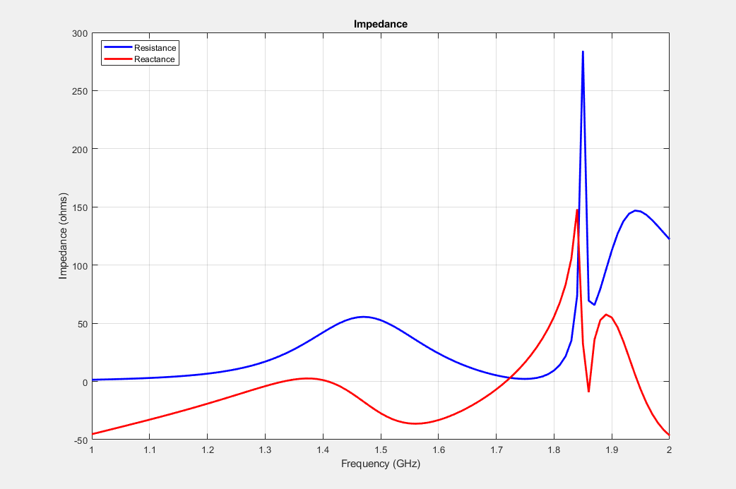
To simulate the Circular Waveguide, the MATLAB Antenna Toolbox(Antenna Designer) was used. To start off the design I selected circular waveguide and inputted a center frequency of 1420MHz. The antenna designer will automatically assign values to the physical dimensions of the antenna to fit the center frequency(how beautiful). Thereafter taking sometime to tune the values of the parameters to deepen the S11 dip to allow for an even better SWR at the specified frequency.  The S11 dips lower when the impedance is at 50 ohms, reactance is at 0 ohms, while the resistive curve stays relatively flat within the local frequency band(meaning it stays close to 50 ohms at the operating frequency.

Construction

The main cylinder is made out of aluminum cylindrical HVAC pipe. The diameter of the pipe will be a unchangeable design constraint, and so I went to the local hardware store and purchased a 6 inch pipe. This was then inputted into the simulator in meters and considering its radius. After conversion the radius is 6.35cm. After playing around with multiple other parameter's of the waveguide and feed point, I came to a final design which centered a S11 dip very close to 1.42GHz. 

Circular Radius: 6.35cm

Cylinder Length: 18cm

Feed Point(from closed end): 14cm

Feed Point(from open end): 4cm

Feed Width: 2.13cm (I used 22 AWG solid core wire in the real design)

The cylinder was cut to a length of 18cm. After cutting the pipe to specified length, the sharp edges along the circumference was smoothen out with a metal file.  One end of the cylinder(farthest from the feed point) was closed off with a few layers of copper tape. The layering was done to ensure sturdiness and durability. A single layer of copper tape was placed along the surface of the cylinder closest to the closed off end of the pipe to conceal the rough tape edges which are from the copper tape used to close off the end of the pipe. A hole of diameter equal to an SMA connector with drilled 14cm away from the copper taped end of the cylinder. The feed was constructed out of a single female SMA connector with a 4.4cm long 22AWG solid core copper wire soldered to the signal pin of the SMA connector. The ground of the SMA connected was securely soldered to the body of the aluminum pipe.

Measurements

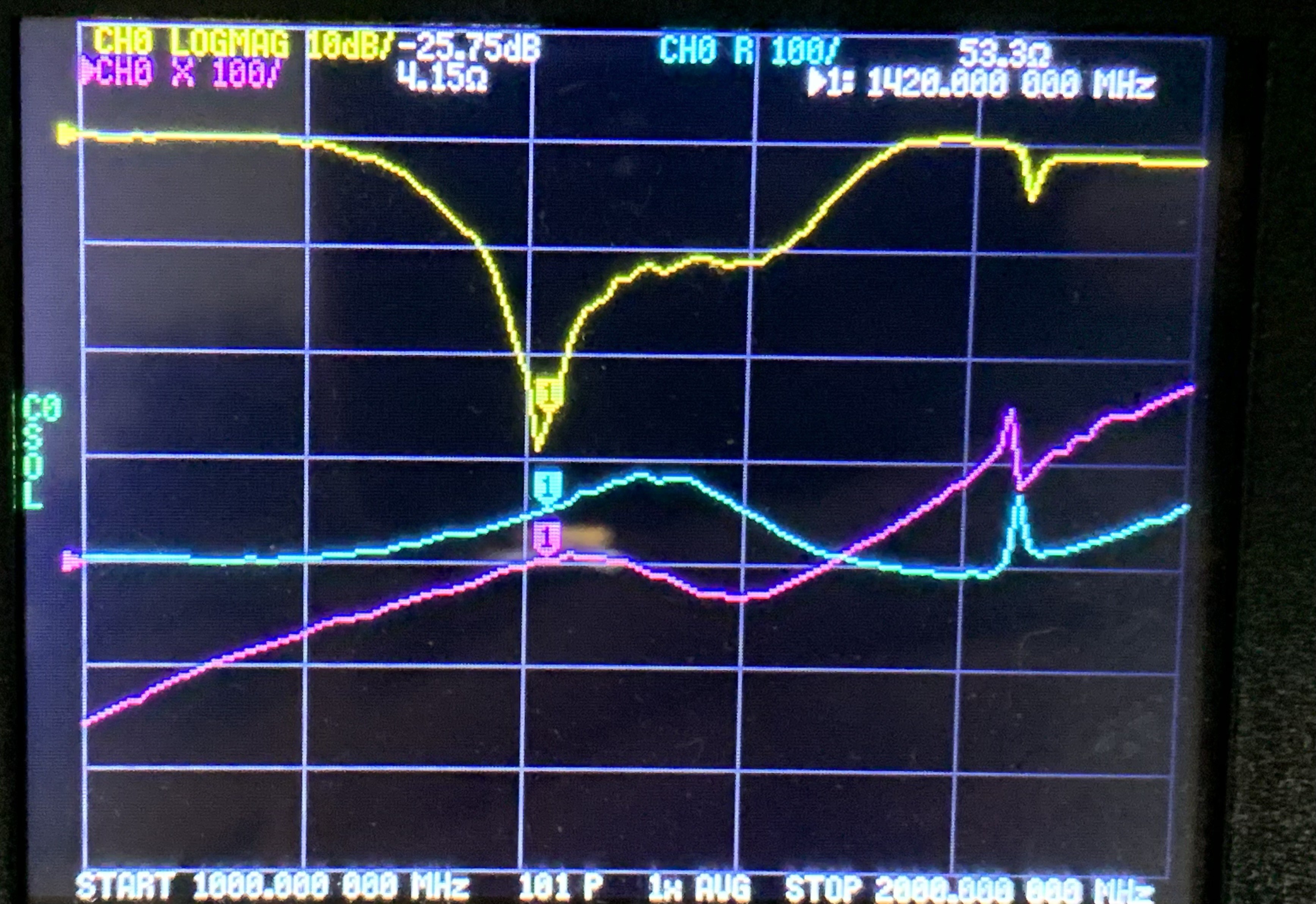
In order to measure the S11 Parameter, Impedance and Resistance of the constructed circular aperture, a NANO VNA will be used. 

Below we can see the measurement setup. The device is calibrated with a small coax cable which was then terminated with: open, short, and 50 ohm load. This calibration is in the frequency range of 1GHz to 2Ghz, the same as the simulated frequency range. We can then compare the two graphs and see if simulation matches measurements! In yellow in the S11 reflection coefficient. Lower values means that more energy is being transmitted, essentially a good antenna. Higher values means that more energy is being reflected back to the source, a bad antenna. In blue is the resistance and in purple is the impedance. 

In this next photo we can get a sense of the antennas directivity and effective aperture. In the photo we can see my hand over the open end of the cylinder, ultimately effecting the dielectric properties of the surrounding space. Remember, the first rule in antennas is that everything effects everything. Notice how the plots on the VNA are dramatically changed when my hand is Infront of the aperture while compared to just open space. Look closely at the VNA in both photos and see how the S11, resistance, and impedance change in the different scenario.