 JTKLENKE
- Goal:
- Create a broadband antenna for voice communications on a military training jet.
- Background:
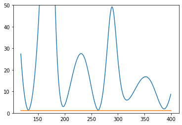
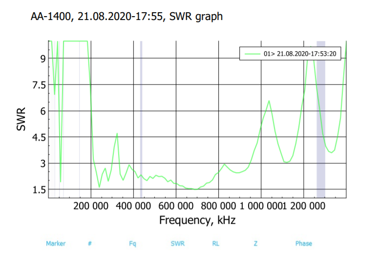
- What is VSWR?
- VSWR stands for Voltage Standing Wave Ratio. It is a measure of how much power is being reflected back to the source from the load. It typically written as a ratio like 2:1 or ∞:1 or as just the first number in that ratio (ie. 2:1 → 2). In a perfect scenario the VSWR would be 1 where 0% of the power is reflected back to the source and is all used by the load. The worst scenario is where 100% of the power is reflected back and this is the VSWR of a short-circuit.
- What are the required specifications?
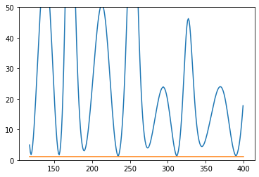
- The VSWR has to be less than or equal to 2.5 for the frequencies of 108MHz to 162MHz and 225MHz to 400MHz but that essentially means that the antenna has to work for the whole range of 108-400.
- The antenna must fit in roughly 27cm tall and 75cm wide space. This makes low-frequency antenna design difficult because the wavelength for the lowest frequencies is 2.7m (though in practice lower because electromagnetic signals travel slower in copper/aluminum)
- What is VSWR?
- Method:
- Options considered:
- brute force/modify existing designs
- computer-optimized antenna design:
- machine-learning options (reinforcement, convolutional, evolutionary, RNN(language processing))
- So far a hybrid of modifying existing designs and computer-optimized seems to be the most efficient and likely to work method.
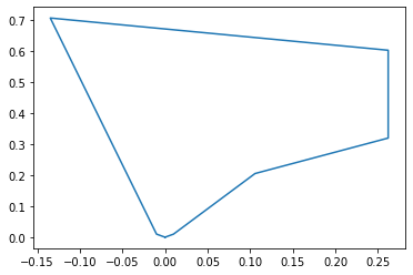
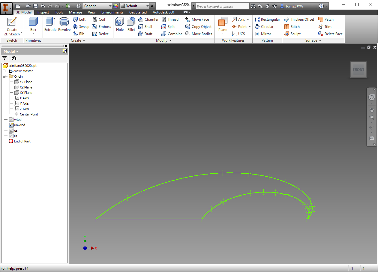
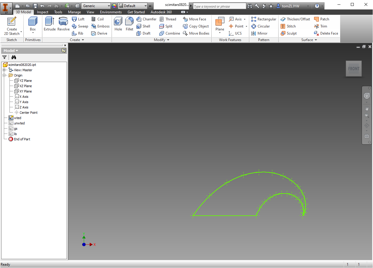
- Using a scimitar antenna design and modifying the parameters, such as scale (k), outside (a1), and inside (a2) curvature, and additional modifications such as vertical and horizontal stretches in conjunction with machine learning to optimize these variables.
- Generalized genetic algorithm
- An algorithm that allows for any antenna that fits the limitations of the space. In practice, this would mean a set/limited count of segments and putting a limit on the points that make up the geometry.
0%
0%
Evolved Broadband Antenna
Using an evolutionary neural network to create an optimized broadband antenna for the ranges of 108MHz to 400MHz
Become a Hackaday.io member
Already have an account? Log in.
Just one more thing
To make the experience fit your profile, pick a username and tell us what interests you.
Pick an awesome username
hackaday.io/
Your profile's URL: hackaday.io/username. Max 25 alphanumeric characters.
Pick a few interests
Projects that share your interests
People that share your interests
 Macrofarad
 freeflightlab
 Cees Meijer