Laser Calibration 2

Laser Power Calibration using Camera

based on camera specifications

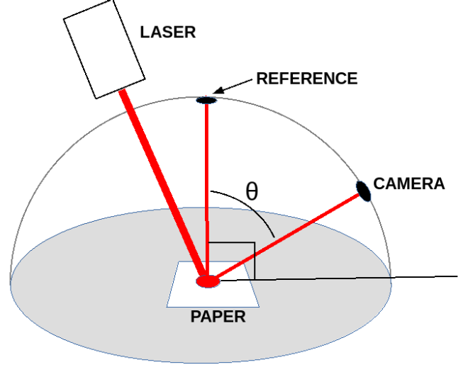
The Equipment Setup

The setup is shown in the image below.

Shining a laser directly into the lens of a camera is probably a bad idea.



By scattering the laser beam and then taking advantage of the inverse square law, we can get any attenuation we want.



A Lambert surface scatters light in a predictable manner. Paper can make a good Lambertian surface. link We had some paper that matched the description of what was used in the link.



We imagine a hemisphere centered on the point at which the laser beam strikes the paper. If we know the radiant flux density (watts per square meter) on the surface of the sphere directly above the paper, we can predict what it should be anywhere else on the surface of the hemisphere.

E' = E cosθ

Where:

E is the radiant flux density on the surface of the hemisphere
   exactly above the middle of our Lambertian surface.
E' is the radiant flux density at the camera lens.
θ is the angle between the reference point and the camera lens

The process will go as follows:

• Calculate the power received by the camera.
• Calculate the power at the reference point on our imaginary hemisphere.
• Figure out how the power on the reference point relates to the laser power.
• Calculate the laser power it took to create the power at the reference point.

Calculate the Power Received by the Camera

The camera was set up such that a picture could be taken of the scattered laser light without saturating.



The aperture was left wide open. The analog gain was set to unity. The exposure time was 1/1000 second.



Full Well Capacity (FWC) = 8180 #taken from Strolls with my Dog



The data from the camera was surprising so a total of four images was taken with the paper being rotated between each image.





The surprise is how much the energy seems to be concentrated in the middle of the laser beam.



Based on an initial guess about the width of the laser beam, the statistical calculations were based on 1 mm cubes.



With the equipment set up as it is, 1 mm at the center of the graduated cylinder is about 14 pixels at the camera.

fwc = 8180. #full well capacity
mdn = 255. #max digital number

f = open("ave.txt", 'r')

total = 0
l = f.readline()
while l != "":
    pos = l.find(" ")
    num = int(l[pos:])
    total = total + num
    l = f.readline()

#that's for an array 15 x 1
#to get a 1 mm square area multiply by 206/15

total = total * 206./15.


f.close()
print(total)
#the red pixels are 1/4 of the total pixels
#to get the correct energy landing on the 1 mm square,
#multiply the electrons by four

electrons = 4 * int(fwc * total / mdn)
print("electrons", electrons)

h = 6.6e-34
c = 3e8

lmbda = 640e-9

ee = h*c/lmbda #electron energy (joules)
print("electron energy", ee, "joules")
eas = electrons * ee #energy at sensor (joules) per 1 mm square
print("energy at sensor", eas, "joules")

The result is:

6743.066666666667
electrons 865228
electron energy 3.09375e-19 joules
energy at sensor 2.676799125e-13 joules

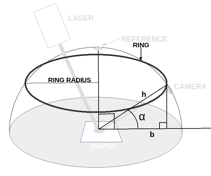
How does the Power at the Reference Point Relate to the Laser Power?

A numerical model was constructed for the hemisphere. The reference point was taken as 1 unit and the power illuminating the surface of the hemisphere was calculated. That provides a ratio between the reference point power and the laser power.



The hemisphere was modelled as a stack of rings of varying radius. The inner surface of each ring was 1 mm wide so the inner surface area of each ring would be 1 mm x 2 * pi * r where r is in mm.





The total power illuminating each ring would be the ring area x cosθ. In the following code, angle α was used to calcualte each ring radius so the power illuminating the ring would be cos(90° - α).

#a set of stacked rings approximating a hemisphere
#the power...

Laser Calibration 1

Laser Power Calibration

If we're going to do anything useful with our test setup, it's necessary to know the power of our laser.



We used four methods to measure the laser power. Each of the methods has its 'issues' but they agree closely enough to give us some confidence in the results.

Light Dependent Resistor (LDR)

We compare the response of a LDR to the laser and to the bright sun.



Why the sun?



The sun is close to being a reliable standard illuminator.



The sun and a low power laser have about the same irradience, approx
imately one milliwatt per square millimeter.



The illumination of the bright sun can be calculated for any time of day, for any day of the year, and for any latitude. link
The resistance of the LDR varies roughly inversely with the power of the incident light.

The Setup

The Light Dependent Resistor (LDR) was mounted behind a 7/64 diameter aperture. When the laser was shone through the apert
ure, the hole was slightly fringed with red light. The intent was that light from the sun and light from the laser would illum
inate the same area on the surface of the LDR.

Results

Resistance due to laser light: 148.2 ohms

Resistance due to sunlight: 20.1 ohms

Sunlight power per square mm: 0.75 mw



laser power = 0.75 x 20.1 / 148.2 = 0.1 mw

Photodiode
compared with bright sunlight

The current of the photodiode is roughly proportional to the number of photons striking it. The sensitive area is a 1 mm s
quare.

Results

Current due to laser light: 0.081 ma

Current due to sunlight: 0.393 ma



laser power = 0.75 x 0.081 / 0.393 = 0.15 mw

Comment

The photodiode has a huge variation in sensitivity across the spectrum of solar radiation. It is highly biased toward the
red end of the visible spectrum and near infrared. This calculation above ignores that fact.

Photodiode
using specifications

The datasheet gives a figure
for quantum yield (0.9 at 850 nm) plus a graph of relative sensitivity vs. wavelength.



For 640 nm (the wavelength of the laser) the electrons generated per photon is: 0.9 x 75% = 0.675.

Calculations

The calculations for this section and the next are based on:

1 - Lumenera

2 - Strolls with my Dog

Strolls with my Dog has done excellent work uncovering the technical details of the Raspberry Pi High Quality Camera.



The following is from a jupyter notebook. It's mostly python3 code but also includes the results of print statements.



#laser wavelength

lmbda = 640e-9

#diode spectral sensitivity per datasheet

ss = 0.75



#measured current (ma)

i = 0.094e-3

#coulomb

cou = 6.24e18

#electrons per second

eps = i * cou

#conversion @ 850 nm electrons per photon

n = 0.9

#photons produced by laser beam

pp = eps / (n * ss)



#energy per photon e = h v = h c / lmbda

h = 6.63e-34

c = 3e8

ep = h * c / lmbda

#energy (watts) = photons per second x energy per photon

pwr = pp * ep

print("Laser Power = ", round(pwr*1000,2), "mw")



Laser Power = 0.27 mw

Using the Camera to Calibrate the Laser

That's sufficiently complicated that it merits its own page. link

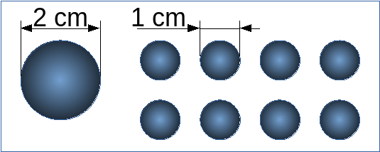
The Effect of Colloid Particle Size

The Effect of Particle Size

h1>The Effect of Particle Size


Compare a large and a small sphere.

The diameter of the large sphere is double that of the small sphere.

The area of the large sphere is four times that of the small sphere.

The volume of the large sphere is eight times that of the small sphere.

It takes eight small spheres to have the same volume as the large sphere.

Compared to the large sphere, the total target area of the small spheres will be (1/4 x 8 = 2) twice
the target area of the big sphere.

So, for a given volume of colloidal particles, the probability of a photon collision changes a lot d
epending on the diameter of the colloidal particles.

The Experiment

We have data for two sets of colloidal dispersions, dilute milk, and diatomaceous earth. We found a
case in which the scattering curves are roughly the same for both.



On those two curves we overlaid a calculated curve for a probability of collision of p = 0.045.



We have reliable data for the size of milk fat particles in 2% homogenized milk (diameter = 0.8 um)
. We used that to calculate the target size for photon collisions. The result was that milk fat partic
les covered 0.047 of the total surface area on which the laser shone. That agrees well with the p = 0.0
45 curve that overlaid the measured scattering curve.



Diatomaceous earth has particle diame
ters ranging from 10 um to 200 um. Based on the match between the curves, we assumed the diluted diatom
aceous earth dispersion had about the same probability of photon collision as the milk and the theoretic
al curves. A particle size with a diameter of 25 um produced that result.



To produce the same scattering as milk fat, diatomaceous earth (DE) required forty times the volume.
(ie. milk fat 0.005 ml in 200 ml water vs. DE 0.2 ml in 200 ml water.) The difference is plausibly e
xplained by the difference in particle size.

Calculations

Python3 code

=====================================



def prn(caption, i):

    print(caption,'{:g}'.format(float('{:.{p}g}'.format(i, p=3))))



from math import pi



#calculate milk, volume of fat in 200 ml

fv = 0.02 * 200



#calculate de volume in 200 ml

dev = 1.25 * 200./250.



#calculate volume of fat in dot00125 solution

dfv = fv * 0.00125



#calculate volume of de in dot2 solution

ddev = dev * 0.2



#prn("dilute volume of fat", dfv, "ml")

#prn("dilute volume of de", ddev, "ml")

prn("dilute volume of fat (ml)", dfv)

prn("dilute volume of de (ml)", ddev)



prn("ddev / dfv", ddev/dfv)



totalMl = 250. #we made 250 ml of fluid

totalMm3 = totalMl * 1000.



deDiaM = 25e-6 #meters

deDiaMm = deDiaM * 1000.

deRadMm = deDiaMm / 2

prn("DE radius (mm)", deRadMm)

totalMl = 250. #we made 250 ml of fluid

totalMm3 = totalMl * 1000.

#deConc = 1.25 ml x 1000 mm3/ml * 200 ml / 250 ml

#started with 250 ml distilled water. cylinder volume = 200 ml

#the sample was diluted with distilled water.

#the undiluted sample was 20% of the final diluted sample

deVolMm3 = 0.2 * (1.25*1000*200./250.) #DE volume in cubic mm of test sample

deVolPerMm3 = deVolMm3 / totalMm3 #DE volume per cubic mm

prn("DE volume per cubic mm", deVolPerMm3)

deSphereVol = (4./3.) * pi * deRadMm**3 #de sphere in cubic mm

prn("DE sphere volume (mm^3)", deSphereVol)

noDeSpMm3 = deVolPerMm3 / deSphereVol #number of DE spheres per cubic mm

prn("number of DE spheres per cubic mm", noDeSpMm3)

deAopS = pi * deRadMm**2 #DE area occluded per sphere in square mm

prn("DE area occluded per sphere (mm^2)", deAopS)

deAo = deAopS * noDeSpMm3

prn("DE area occluded", deAo)



mfDiaM = 0.8e-6 #meters

mfDiaMm = mfDiaM * 1000.

mfRadMm = mfDiaMm / 2

prn("milk fat radius (mm)", mfRadMm)

totalMl = 200. #200 ml sample in graduated cylinder

totalMm3 = totalMl * 1000.

#from above, volume of milk fat in dilute solution = dfv

mfVolPerMm3 = 1000 * dfv / totalMm3 #DE volume per cubic mm

prn("milk fat volume per cubic mm", mfVolPerMm3)

mfSphereVol = (4./3.) * pi * mfRadMm**3 #mf sphere in cubic mm

prn("milk fat sphere volume (mm^3)", mfSphereVol)

noMfSpMm3 = mfVolPerMm3 / mfSphereVol #number of milk fat spheres...